TL;DR#
Reinforcement learning (RL) agents often struggle to generalize across tasks with varying environmental features requiring different optimal behaviors (skills). Existing context encoders based on contrastive learning, while improving generalization, suffer from the ’log-K curse,’ requiring massive datasets. This limits their real-world applicability.
This paper introduces Skill-aware Mutual Information (SaMI), an optimization objective that helps distinguish context embeddings based on skills, and Skill-aware Noise Contrastive Estimation (SaNCE), a more efficient estimator for SaMI. Experiments on modified MuJoCo and Panda-gym benchmarks demonstrate that RL agents learning with SaMI achieve substantially improved zero-shot generalization to unseen tasks, showing greater robustness to smaller datasets and potentially overcoming the log-K curse.
Key Takeaways#
Why does it matter?#
This paper is important because it tackles the challenge of improving generalization in reinforcement learning, a crucial issue limiting the applicability of RL in complex real-world scenarios. By introducing a novel skill-aware objective function and a data-efficient estimator, the research offers a promising solution to enhance zero-shot generalization and overcome the limitations of existing methods. This opens up new avenues for research in meta-reinforcement learning and its applications in robotics and other domains.
Visual Insights#
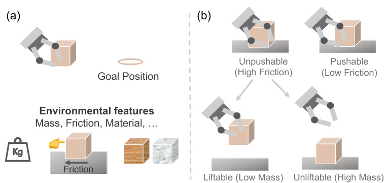
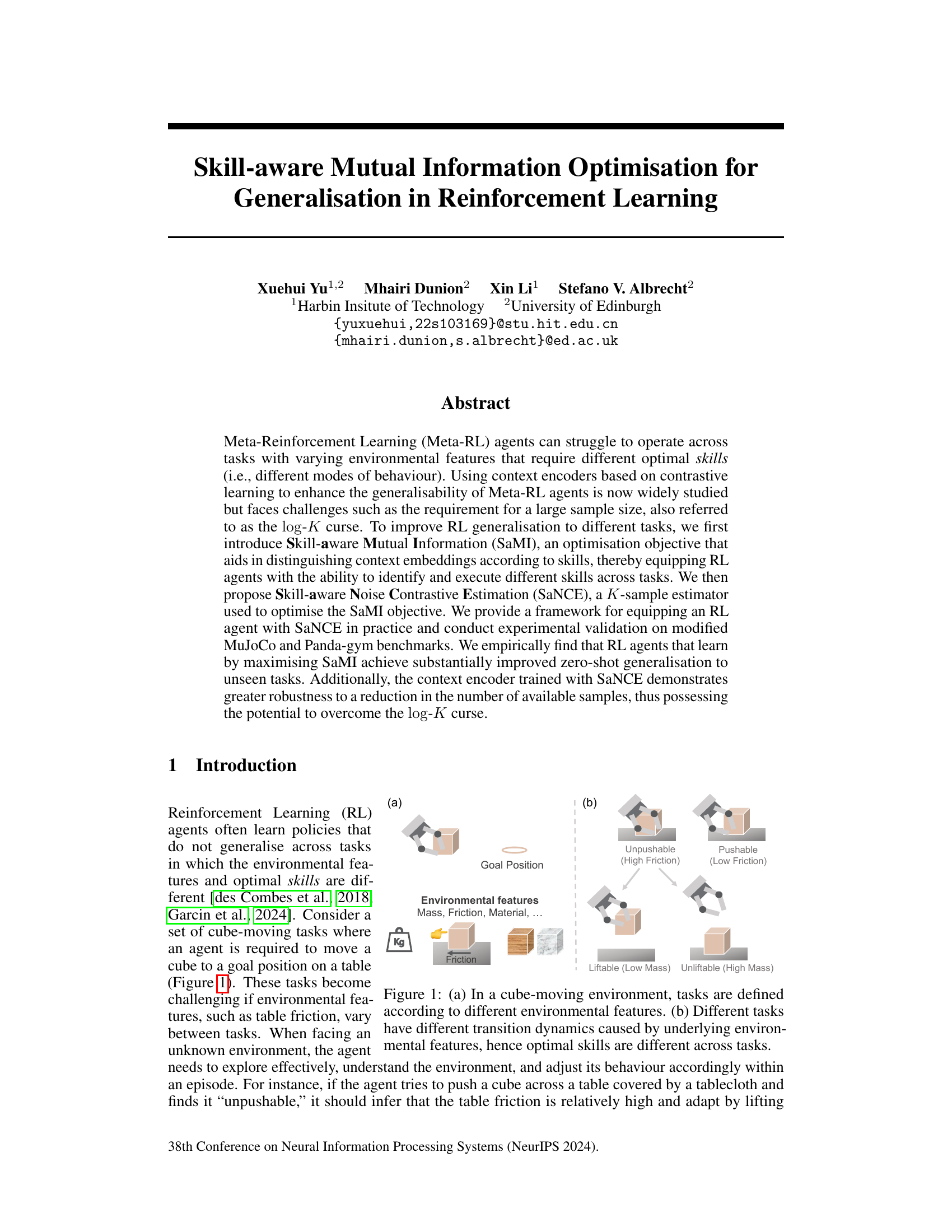
🔼 This figure illustrates the concept of skill-aware generalization in reinforcement learning using a cube-moving task as an example. (a) shows that tasks can be defined by varying environmental factors, such as table friction or cube mass. (b) shows how these factors lead to different optimal ways (skills) of solving the task. For example, a high-friction surface might require lifting the cube, while a low-friction surface would allow for pushing. The agent needs to learn to identify and adapt its behaviour to these different conditions.
read the caption
Figure 1: (a) In a cube-moving environment, tasks are defined according to different environmental features. (b) Different tasks have different transition dynamics caused by underlying environmental features, hence optimal skills are different across tasks.
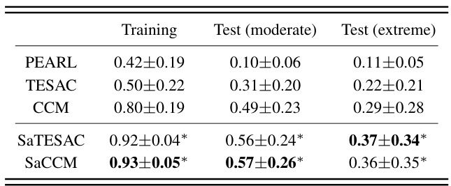
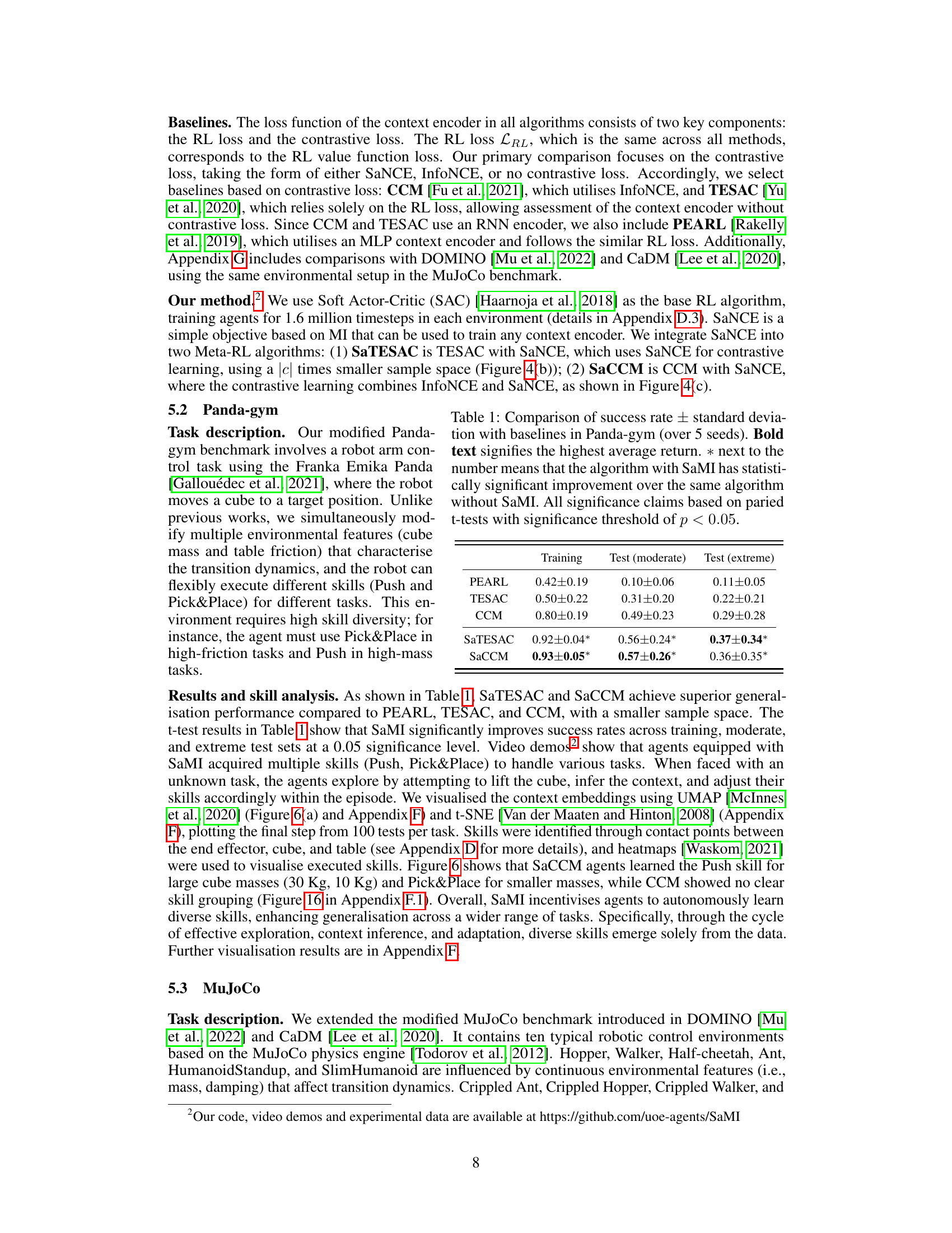
🔼 This table compares the success rates of different meta-reinforcement learning algorithms on the Panda-gym benchmark. It shows the performance of four baselines (PEARL, TESAC, CCM) and two proposed methods (SaTESAC, SaCCM) across training, moderate test, and extreme test scenarios. The * indicates statistically significant improvements compared to the same algorithm without the SaMI optimization.
read the caption
Table 1: Comparison of success rate ± standard deviation with baselines in Panda-gym (over 5 seeds). Bold text signifies the highest average return. * next to the number means that the algorithm with SaMI has statistically significant improvement over the same algorithm without SaMI. All significance claims based on paired t-tests with significance threshold of p < 0.05.
In-depth insights#
SaMI: Skill-Aware MI#
The proposed SaMI (Skill-Aware Mutual Information) framework offers a novel approach to enhance generalization in reinforcement learning. SaMI cleverly integrates the concept of skills into the mutual information objective function. This crucial modification allows the model to learn context embeddings that are not only discriminative across different tasks, but also explicitly linked to specific skills required for task completion. By maximizing SaMI, the RL agent implicitly learns to distinguish between situations that demand diverse skills. This results in improved zero-shot generalization and a more robust contextual understanding, enabling better adaptation to unseen tasks and environments. SaNCE (Skill-Aware Noise Contrastive Estimation), the proposed estimator for SaMI, further enhances sample efficiency. This is particularly relevant for reinforcement learning, as large datasets are often hard to obtain. The effectiveness of SaMI is demonstrated empirically through experiments on modified MuJoCo and Panda-gym benchmarks, showcasing improved performance over existing Meta-RL algorithms.
SaNCE: Data-Efficient Estimator#
The proposed Skill-aware Noise Contrastive Estimation (SaNCE) method offers a data-efficient approach to estimating mutual information (MI) within the context of meta-reinforcement learning. SaNCE directly addresses the ’log-K curse’, a common challenge in traditional MI estimation methods, by significantly reducing the number of samples required for accurate estimation. This is achieved by strategically sampling trajectories based on distinct skills, thereby focusing the learning process on skill-relevant information and reducing the need for extensive negative sampling. SaNCE’s skill-aware sampling strategy further enhances efficiency by autonomously acquiring relevant skills directly from the data, eliminating the need for pre-defined skill distributions. This data efficiency is crucial for meta-RL, where obtaining large amounts of data can be challenging. Empirical validation on MuJoCo and Panda-gym benchmarks demonstrated SaNCE’s superior performance compared to standard MI estimators and enhanced generalization to unseen tasks, highlighting its potential to improve the robustness and sample efficiency of meta-RL agents.
Benchmark Analyses#
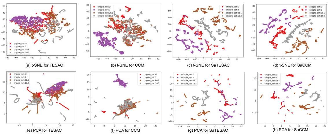
A robust benchmark analysis is crucial for evaluating the effectiveness of new reinforcement learning (RL) methods. It should involve a diverse set of tasks that thoroughly test the algorithm’s ability to generalize. The selection of benchmark environments is critical, needing to span different complexities and characteristics. Using established benchmarks like MuJoCo and Panda-Gym allows for comparison against existing state-of-the-art approaches. Quantifiable metrics like average return and success rate, across various difficulty levels (e.g., moderate and extreme), provide concrete measures of performance. A thoughtful analysis should discuss the reasons behind successes and failures, linking performance to specific properties of the tasks and the algorithm’s design. Visualizations, such as UMAP and t-SNE, can offer valuable insights into learned representations and skill acquisition. The comparison should extend beyond simple numerical results; qualitative observations and insightful interpretations are essential to draw meaningful conclusions. Analyzing the impact of hyperparameters, particularly those controlling the balance between contrastive and reinforcement learning objectives, is another significant factor. A robust analysis will discuss the algorithm’s sample efficiency, its sensitivity to parameter choices and its ability to overcome limitations such as the log-K curse. Ultimately, a compelling benchmark analysis should not just present results, but should also provide a comprehensive and nuanced understanding of the proposed method’s strengths and weaknesses.
Log-K Curse Mitigation#
The ’log-K curse’ is a significant challenge in contrastive learning and meta-reinforcement learning (meta-RL), stemming from the use of K-sample estimators to approximate mutual information (MI). These estimators’ accuracy degrades as the number of samples (K) increases, necessitating massive datasets. This paper tackles the curse by introducing Skill-aware Mutual Information (SaMI), a modified MI objective focusing on skill-related information rather than indiscriminately comparing all trajectories. This refinement, coupled with the proposed Skill-aware Noise Contrastive Estimation (SaNCE), a more sample-efficient K-sample estimator, leads to superior performance even with smaller datasets. SaNCE’s sample-efficient nature makes it particularly attractive in data-scarce RL environments, showcasing a path toward alleviating the log-K curse limitations, thereby improving the generalization of meta-RL agents.
Future Work#
The paper’s conclusion suggests promising avenues for future research. Extending SaMI to handle interdependent environmental features is crucial, as real-world scenarios rarely present independent variables. The current SaMI framework assumes some level of independence, limiting its applicability to complex settings. Therefore, investigating how to modify SaMI to effectively handle correlations between variables is vital. Furthermore, exploring a model-based approach to SaMI is recommended. The current method uses model-free RL, but a model-based approach could offer advantages, particularly when dealing with dynamic environments where the transition function changes frequently. This suggests a shift towards integrating model-based RL with SaMI, which could improve efficiency and generalizability. Lastly, testing SaMI and SaNCE on more complex and realistic tasks is needed to solidify their effectiveness in real-world scenarios. This includes evaluating the algorithms on tasks requiring more sophisticated skills and larger state spaces, moving beyond the benchmarks presented in the paper. Such rigorous testing will help to validate SaMI and SaNCE’s generalizability and robustness.
More visual insights#
More on figures

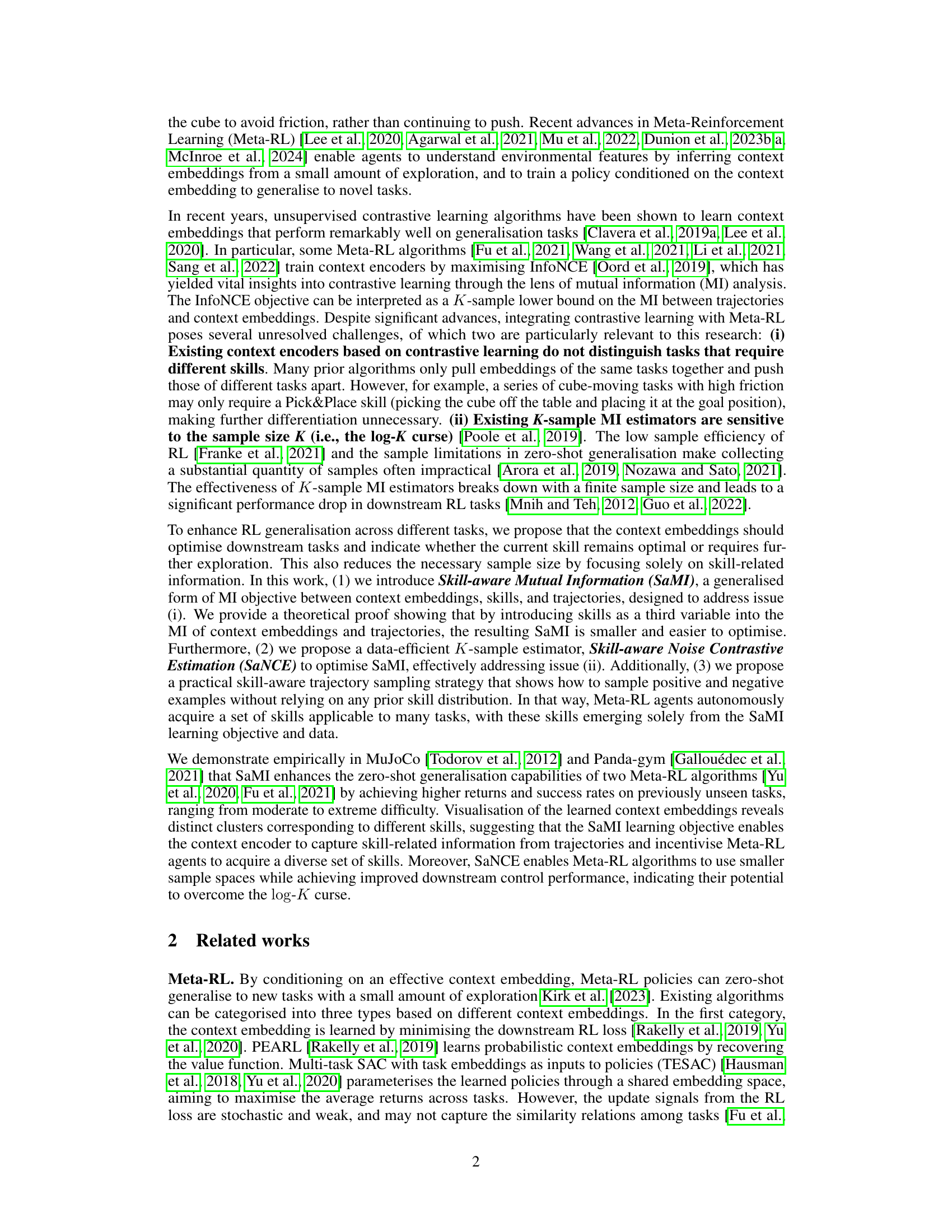
🔼 This figure illustrates how a policy conditioned on a fixed context embedding represents a specific skill. It shows two examples: the ‘Push’ skill, where the agent pushes the cube across the table, and the ‘Pick&Place’ skill, where the agent picks up the cube and places it at the goal position. The context embedding acts as a selector for the skill, demonstrating how different skills are encoded within the context embedding space.
read the caption
Figure 2: A policy π conditioned on a fixed context embedding c is defined as a skill π(·|c) (shortened as πc). The policy π conditioned on a fixed c alters the state of the environment in a consistent way, thereby exhibiting a mode of skill. The skill π(c1) moves the cube on the table in trajectory T and is referred to as the Push skill; correspondingly, the Pick&Place skill π(c2) takes the cube off the table and places it in the goal position in the trajectory T.

🔼 The figure shows the convergence speed of different mutual information estimators. I(c; τc) represents the true mutual information between context embeddings (c) and trajectories (τc). IInfoNCE(c; πc; τc) is a K-sample estimator for MI which has a logarithmic upper bound (logK), shown as a horizontal gray line. Because of its loose lower bound, IInfoNCE converges to logK slowly. IsaMI(c; πc; τc) is a tighter lower bound than IInfoNCE and converges more quickly. SaNCE is a proposed estimator that more closely approximates IsaMI, resulting in the fastest convergence.
read the caption
Figure 3: IInfoNCE(C;;Te), with a finite sample size of K, is a loose lower bound of I(C; Tc) and leads to lower performance embeddings. IsaMI (C; πc; Te) is a lower ground-truth MI, and ISaNCE (C; c; Tc) is a tighter lower bound.

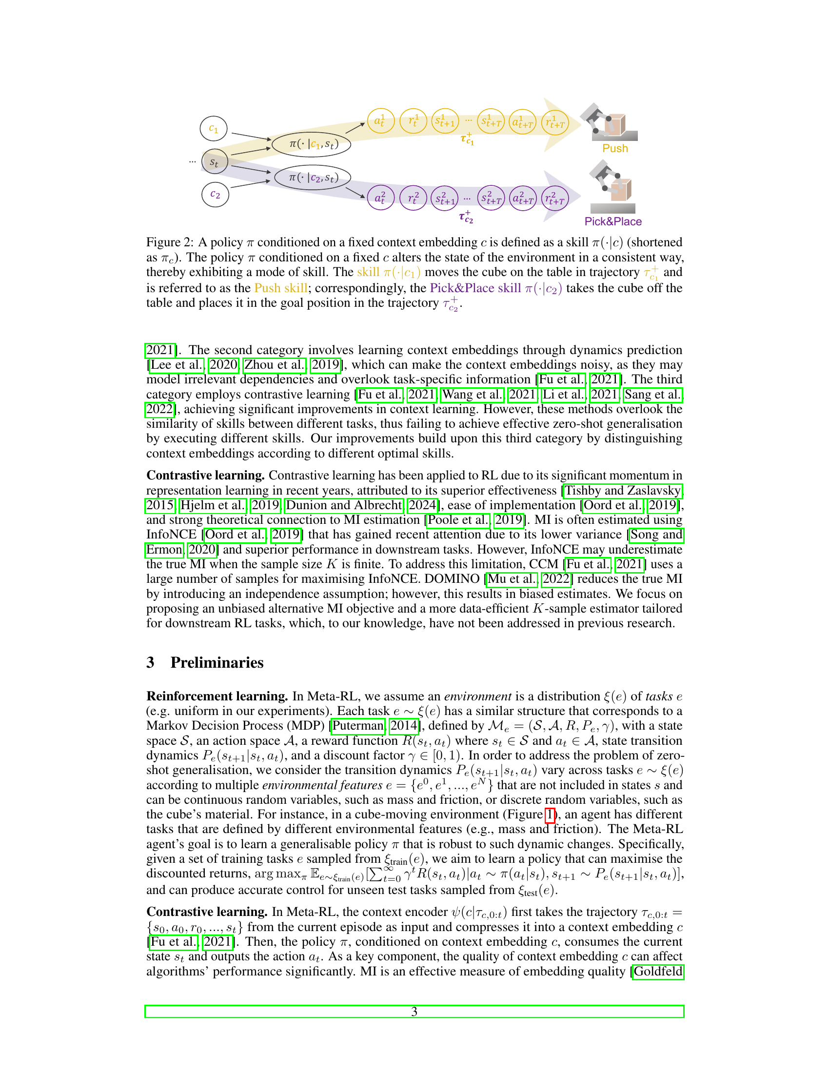
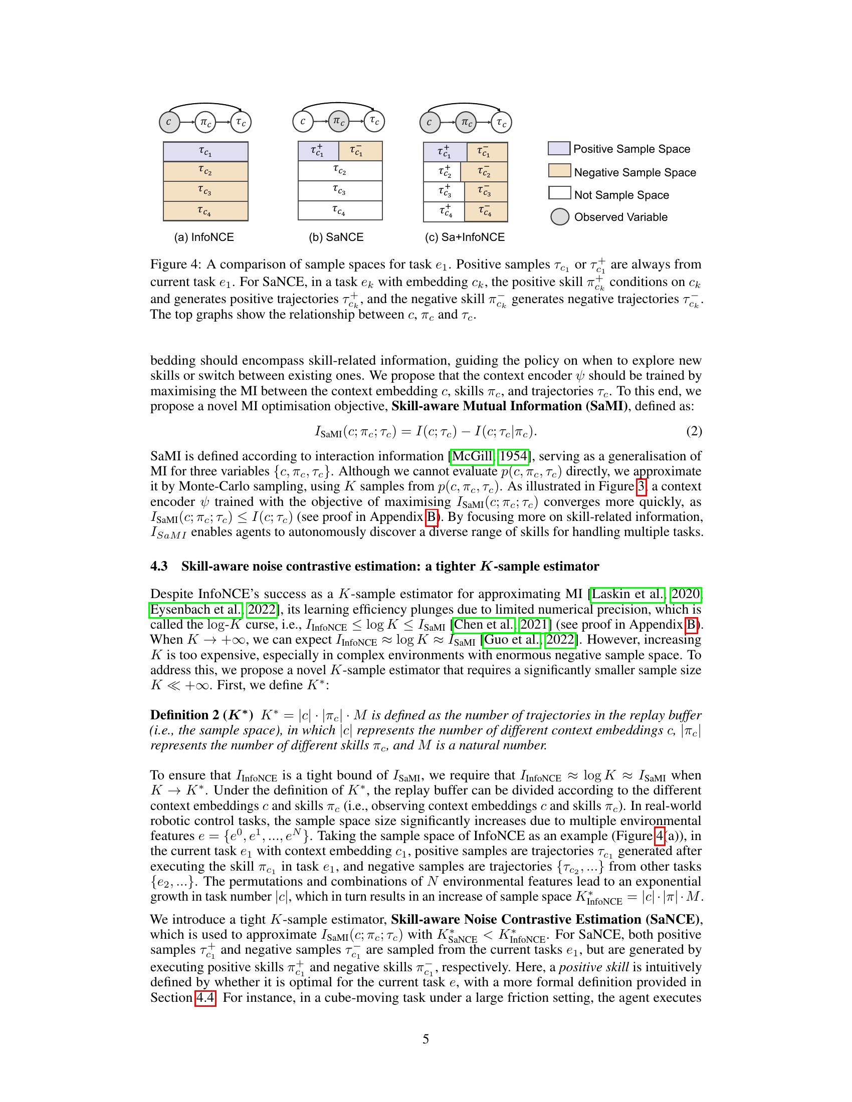
🔼 This figure compares three different sampling strategies for contrastive learning in the context of meta-reinforcement learning. (a) InfoNCE samples positive examples from the current task and negative examples from all other tasks. (b) SaNCE samples both positive and negative examples from the current task, but distinguishes them based on skills. (c) Sa+InfoNCE combines the strategies of InfoNCE and SaNCE. The figure illustrates the different sample spaces used by each method and highlights the key difference of SaNCE in focusing on skill-related information within the current task to improve sample efficiency.
read the caption
Figure 4: A comparison of sample spaces for task e1. Positive samples Te₁ or T are always from current task e₁. For SaNCE, in a task ek with embedding ck, the positive skill πc conditions on ck and generates positive trajectories Tπc, and the negative skill πc generates negative trajectories Tπc. The top graphs show the relationship between c, πc and Tc.

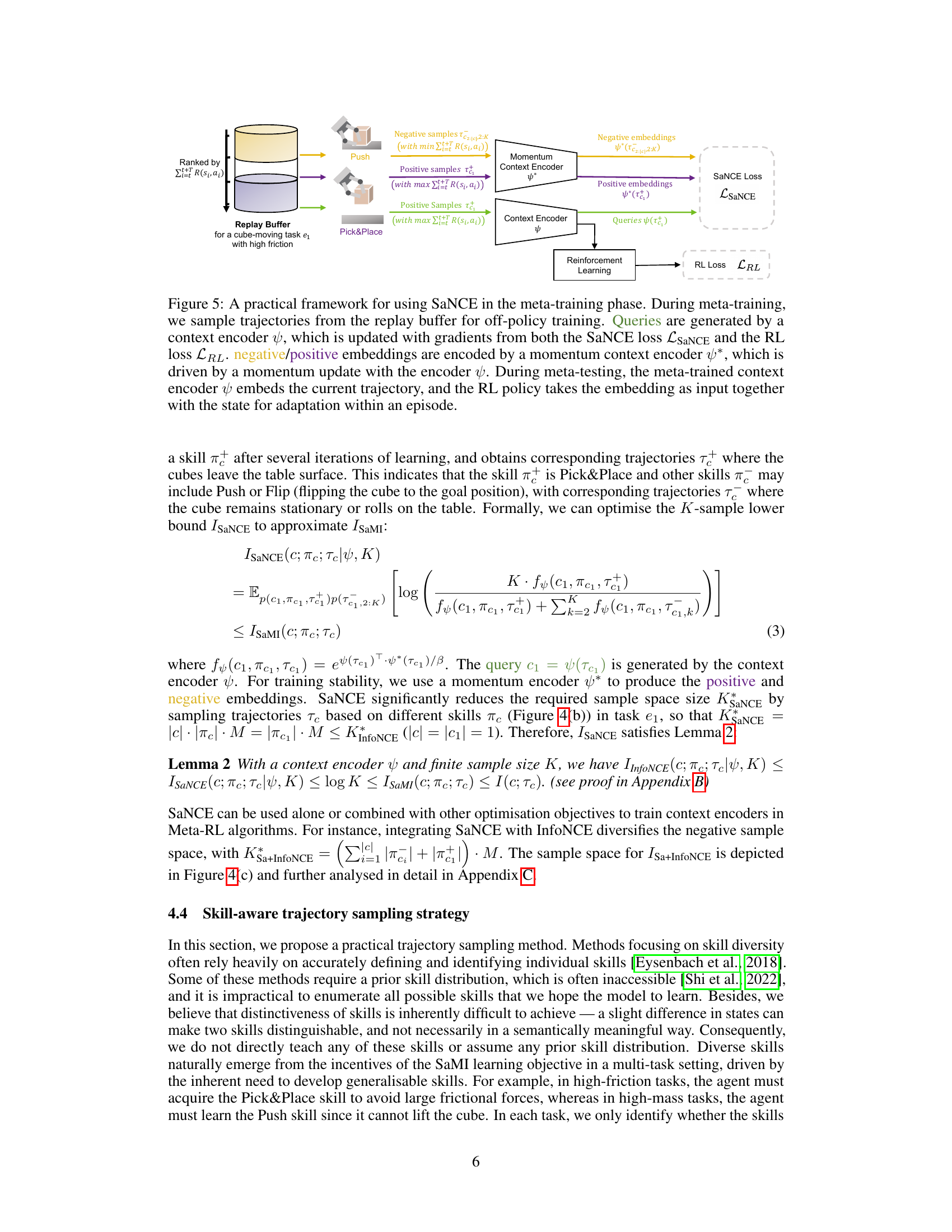
🔼 This figure shows a practical framework for integrating SaNCE into the meta-training process. It details how trajectories are sampled from a replay buffer, how a context encoder and momentum encoder generate queries and positive/negative embeddings, and how the encoder is updated using both SaNCE and RL loss functions. The meta-testing phase is also briefly depicted, showing how the trained context encoder is used for adaptation during an episode.
read the caption
Figure 5: A practical framework for using SaNCE in the meta-training phase. During meta-training, we sample trajectories from the replay buffer for off-policy training. Queries are generated by a context encoder ψ, which is updated with gradients from both the SaNCE loss LSaNCE and the RL loss LRL. negative/positive embeddings are encoded by a momentum context encoder ψ*, which is driven by a momentum update with the encoder ψ. During meta-testing, the meta-trained context encoder ψ embeds the current trajectory, and the RL policy takes the embedding as input together with the state for adaptation within an episode.

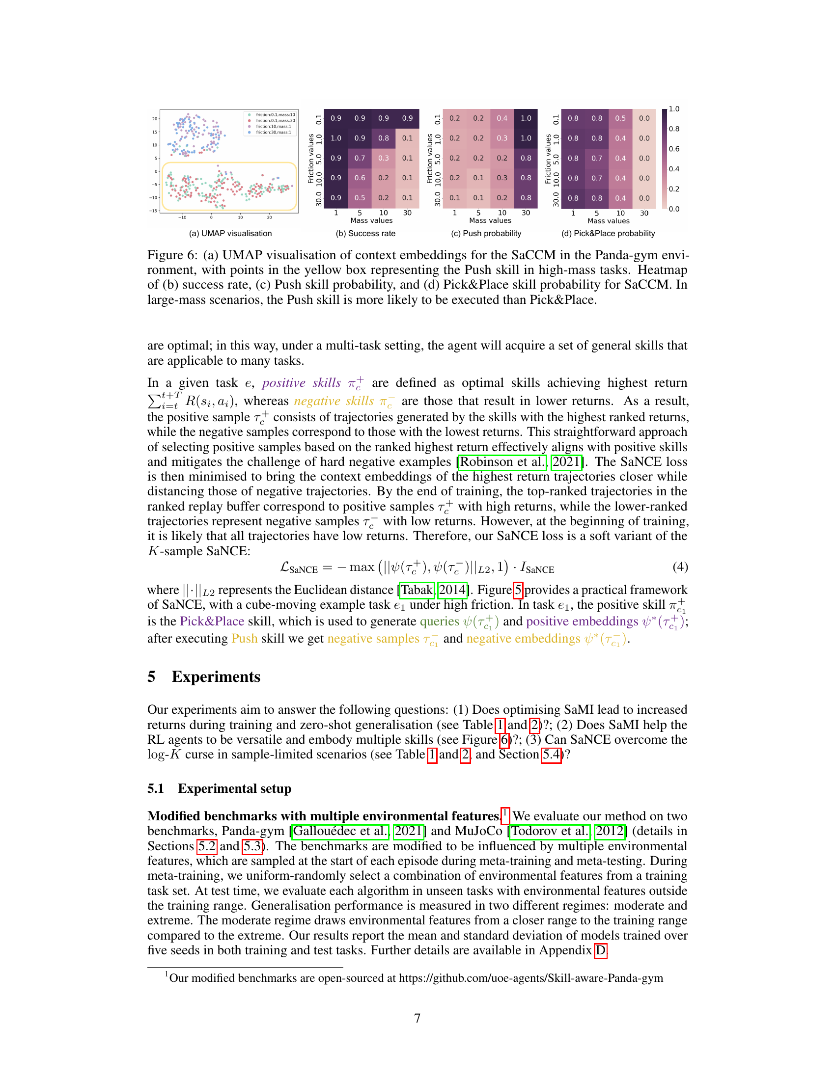
🔼 This figure visualizes context embeddings learned by SaCCM in the Panda-gym environment using UMAP. The yellow box highlights the Push skill in high-mass scenarios. Heatmaps then show the success rate, probability of using the Push skill, and probability of using the Pick&Place skill across various mass and friction conditions. It demonstrates that SaCCM learns to associate different skills with different environmental conditions (mass and friction in this case).
read the caption
Figure 6: (a) UMAP visualisation of context embeddings for the SaCCM in the Panda-gym environment, with points in the yellow box representing the Push skill in high-mass tasks. Heatmap of (b) success rate, (c) Push skill probability, and (d) Pick&Place skill probability for SaCCM. In large-mass scenarios, the Push skill is more likely to be executed than Pick&Place.

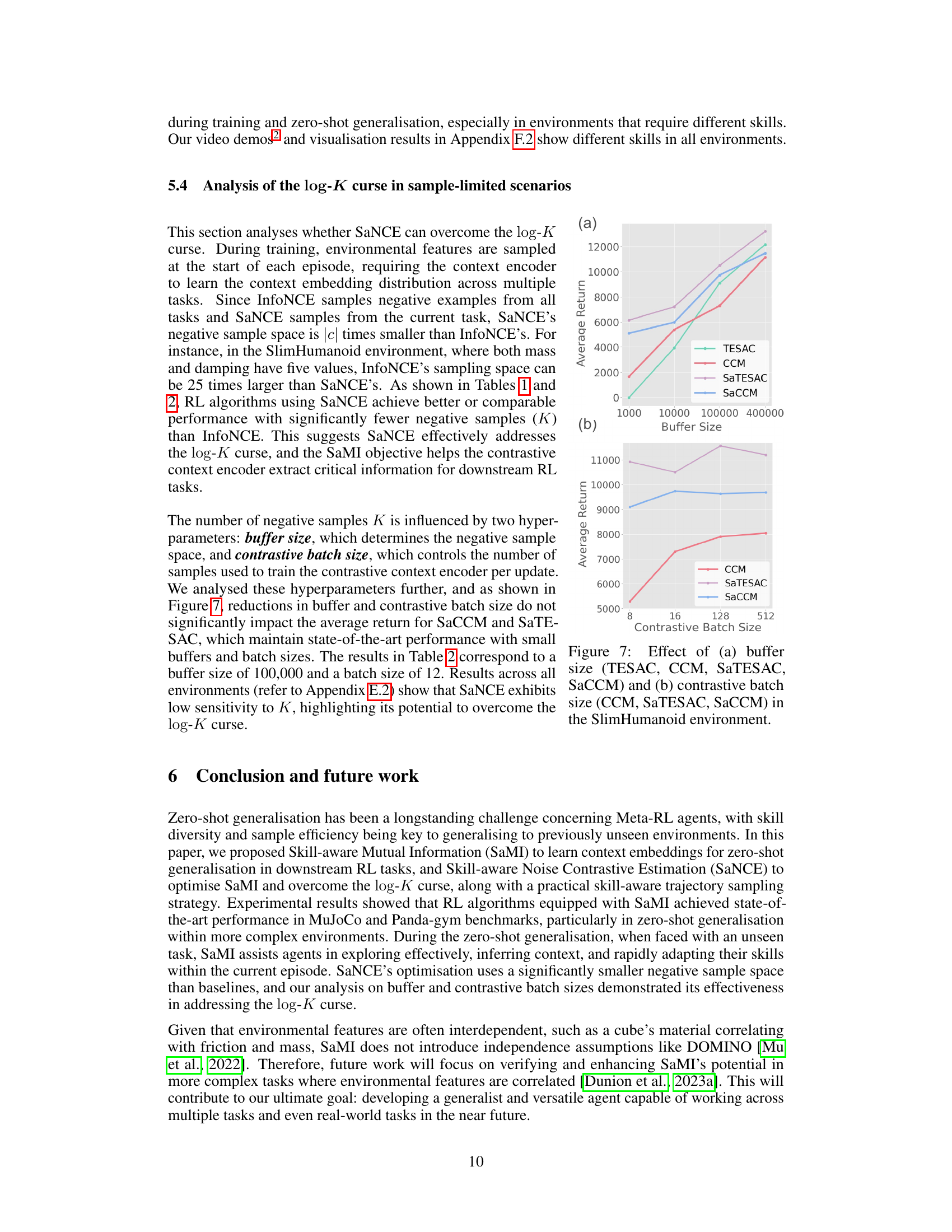
🔼 The figure shows the effect of buffer size and contrastive batch size on the performance of different algorithms in the SlimHumanoid environment. (a) shows how average return varies with different buffer sizes (400000, 100000, 10000, and 1000) for TESAC, CCM, SaTESAC, and SaCCM. (b) shows how average return varies with different contrastive batch sizes (512, 128, 16, and 8) for CCM, SaTESAC, and SaCCM.
read the caption
Figure 7: Effect of (a) buffer size (TESAC, CCM, SaTESAC, SaCCM) and (b) contrastive batch size (CCM, SaTESAC, SaCCM) in the SlimHumanoid environment.

🔼 This figure uses Venn diagrams to illustrate the concepts of mutual information and interaction information, and also shows a graphical representation of the causal relationship between context embedding, skill, and trajectory in a meta-RL setting. Panel (a) shows the mutual information between the context embedding and trajectory. Panel (b) depicts the interaction information which is the difference between the mutual information of context embedding and trajectory and the conditional mutual information of the context embedding and trajectory given the skill. Panel (c) represents a causal graphical model showing the context embedding as a common cause influencing both the skill and the trajectory.
read the caption
Figure 8: Venn diagrams illustrating (a) mutual information I(c; τc), (b) interaction information IsaMI(C; πc; τc), and (c) the MDP graph of the context embedding c, skill πc, and trajectory τc, which represents a common-cause structure [Neuberg, 2003].
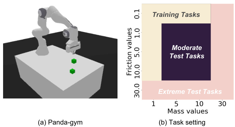
🔼 This figure shows the modified Panda-gym environment used in the experiments. Panel (a) is a 3D rendering of the robotic arm and cube setup. Panel (b) is a heatmap showing the ranges of mass and friction values used to define the training and testing tasks. The training tasks are in the central region of the plot, the moderate test tasks are in a region adjacent to the training tasks, and the extreme test tasks cover unseen areas.
read the caption
Figure 9: (a) Modified Panda-gym benchmarks, (b) the training tasks, moderate test tasks, and extreme test tasks. The moderate test task setting involves combinatorial interpolation, while the extreme test task setting includes unseen ranges of environmental features and represents an extrapolation.
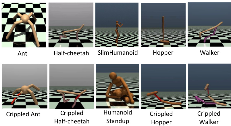
🔼 This figure shows the ten different robotic control environments used in the modified MuJoCo benchmark. These environments include variations of Ant, Half-Cheetah, SlimHumanoid, Hopper, and Walker robots, along with crippled versions of the Ant, Half-Cheetah, and Walker, as well as the Humanoid Standup. These variations are used to evaluate the generalization capability of the reinforcement learning agents across tasks with varying difficulty and characteristics.
read the caption
Figure 10: Ten environments in modified MuJoCo benchmark.
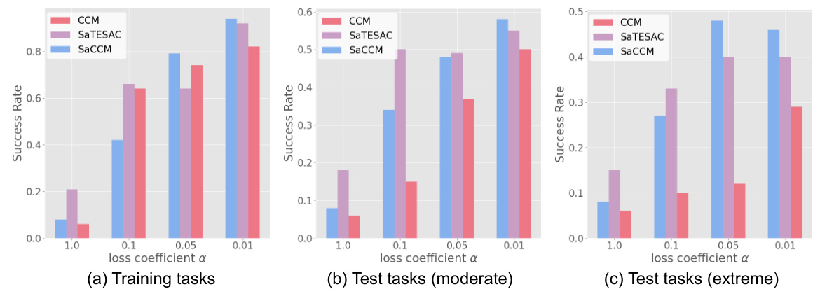
🔼 This figure shows the impact of the loss coefficient α on the performance of three algorithms (CCM, SaTESAC, and SaCCM) across different settings: training tasks, moderate test tasks, and extreme test tasks. The x-axis represents different values of α, and the y-axis represents the success rate. The figure illustrates how the choice of α affects the success rate in these three scenarios.
read the caption
Figure 11: Loss coefficient α analysis of Panda-gym benchmark in training and test (moderate and extreme) tasks.

🔼 This figure visualizes the context embeddings learned by the SaCCM model in the Panda-gym environment using UMAP. The yellow box highlights embeddings associated with the ‘Push’ skill, prevalent in tasks involving high-mass cubes. The heatmaps further illustrate the success rate and probability of using either the ‘Push’ or ‘Pick&Place’ skill across different combinations of cube mass and table friction. The results demonstrate that SaCCM effectively learns to associate context embeddings with specific skills, adapting its strategy based on task characteristics.
read the caption
Figure 6: (a) UMAP visualisation of context embeddings for the SaCCM in the Panda-gym environment, with points in the yellow box representing the Push skill in high-mass tasks. Heatmap of (b) success rate, (c) Push skill probability, and (d) Pick&Place skill probability for SaCCM. In large-mass scenarios, the Push skill is more likely to be executed than Pick&Place.

🔼 This figure illustrates the concept of skill-aware generalization in reinforcement learning. Panel (a) shows a cube-moving task with varying environmental features such as friction and mass, leading to different optimal skills (modes of behaviour) for each task. Panel (b) highlights how these differing environmental features result in varying transition dynamics and, consequently, the need for different skills (e.g., pushing versus lifting) to succeed.
read the caption
Figure 1: (a) In a cube-moving environment, tasks are defined according to different environmental features. (b) Different tasks have different transition dynamics caused by underlying environmental features, hence optimal skills are different across tasks.

🔼 This figure compares the sample spaces used for training the context encoder in three different methods: InfoNCE, SaNCE, and a combination of both. InfoNCE uses positive samples from the current task and negative samples from other tasks, while SaNCE only uses samples from the current task, distinguishing positive and negative samples based on the skill used. The combined method utilizes both strategies. The figure illustrates the different sample spaces visually and highlights the key differences between the approaches.
read the caption
Figure 4: A comparison of sample spaces for task e1. Positive samples Te₁ or T are always from current task e₁. For SaNCE, in a task ek with embedding ck, the positive skill πc conditions on ck and generates positive trajectories Tπc, and the negative skill πc generates negative trajectories Tπc. The top graphs show the relationship between c, πc and Tc.
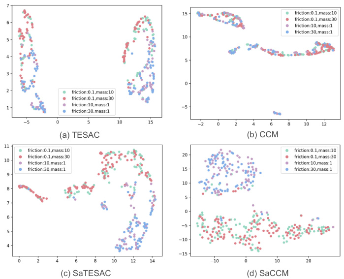
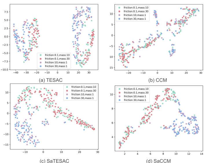
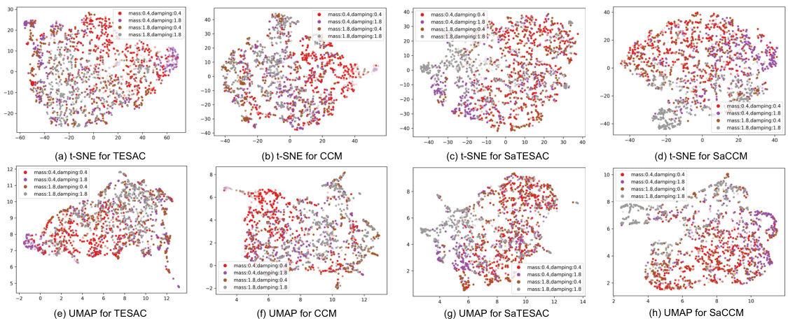
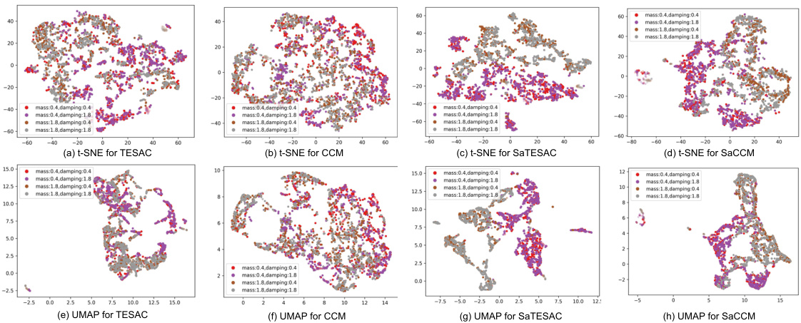
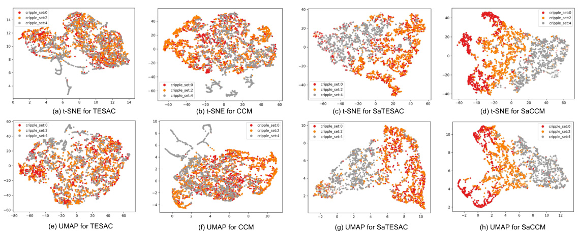
🔼 UMAP visualization of context embeddings for TESAC, CCM, SaTESAC, and SaCCM algorithms in the Panda-gym environment. Each point represents a trajectory. The plots show how different algorithms cluster trajectories based on the underlying skills (Push and Pick&Place). SaMI-based algorithms (SaTESAC and SaCCM) show more distinct clustering than TESAC and CCM, indicating better skill separation.
read the caption
Figure 15: UMAP visualisation of context embeddings extracted from trajectories collected in the Panda-gym environments.
🔼 This figure visualizes the context embeddings learned by SaCCM in the Panda-gym environment using UMAP. It shows how the learned embeddings cluster based on the skills (Push and Pick&Place) employed by the agent, particularly highlighting the preference for the Push skill in high-mass scenarios. Heatmaps further illustrate the success rate and the probabilities of using each skill under different mass and friction conditions.
read the caption
Figure 6: (a) UMAP visualisation of context embeddings for the SaCCM in the Panda-gym environment, with points in the yellow box representing the Push skill in high-mass tasks. Heatmap of (b) success rate, (c) Push skill probability, and (d) Pick&Place skill probability for SaCCM. In large-mass scenarios, the Push skill is more likely to be executed than Pick&Place.

🔼 This figure compares the sample spaces used by InfoNCE and SaNCE for training a context encoder. InfoNCE uses positive samples from the current task and negative samples from other tasks, while SaNCE only uses samples from the current task, with positive samples from positive skills and negative samples from negative skills. The figure illustrates how SaNCE reduces the size of the negative sample space by focusing on skill-related information.
read the caption
Figure 4: A comparison of sample spaces for task e1. Positive samples Te₁ or T are always from current task e₁. For SaNCE, in a task ek with embedding ck, the positive skill πc conditions on ck and generates positive trajectories Tπc, and the negative skill πc generates negative trajectories Tπc. The top graphs show the relationship between c, πc and Tc.

🔼 This figure compares the sample spaces used by InfoNCE and SaNCE for training a context encoder in a meta-reinforcement learning setting. InfoNCE uses positive samples from the current task and negative samples from other tasks. SaNCE, in contrast, utilizes both positive and negative samples from the current task, but distinguishes them based on the skill used to generate them. SaNCE’s approach is shown to be more data-efficient.
read the caption
Figure 4: A comparison of sample spaces for task e1. Positive samples Te₁ or T are always from current task e₁. For SaNCE, in a task ek with embedding ck, the positive skill πc conditions on ck and generates positive trajectories Tπc, and the negative skill π generates negative trajectories Tπc. The top graphs show the relationship between c, πc and Tc.
🔼 This figure compares the sample spaces used by InfoNCE and SaNCE for training a context encoder. InfoNCE uses samples from different tasks to distinguish between tasks. In contrast, SaNCE, which focuses on skills, samples trajectories from the same task but uses different skills to create positive and negative samples for comparison. The goal is to show how SaNCE can use a smaller sample space to learn an effective context embedding by focusing on skill-related information.
read the caption
Figure 4: A comparison of sample spaces for task e1. Positive samples Te₁ or T are always from current task e₁. For SaNCE, in a task ek with embedding ck, the positive skill πc conditions on ck and generates positive trajectories Tπc, and the negative skill πc generates negative trajectories Tπc. The top graphs show the relationship between c, πc and Tc.

🔼 This figure compares three different sampling strategies for contrastive learning in meta-reinforcement learning: InfoNCE, SaNCE, and Sa+InfoNCE. Each strategy differs in how it samples positive and negative examples for training a context encoder. InfoNCE samples positive examples from the current task and negative examples from all other tasks. SaNCE samples both positive and negative examples from the current task, but the positive samples come from the optimal skill for the task, while negative examples come from suboptimal skills. Sa+InfoNCE combines both InfoNCE and SaNCE sampling strategies. The figure illustrates the different sample spaces for each strategy, highlighting the differences in sample size and diversity.
read the caption
Figure 4: A comparison of sample spaces for task e1. Positive samples Te₁ or T are always from current task e₁. For SaNCE, in a task ek with embedding ck, the positive skill πc conditions on ck and generates positive trajectories Tπc, and the negative skill π generates negative trajectories Tπc. The top graphs show the relationship between c, πc and Tc.

🔼 This figure compares the sample spaces used by InfoNCE and SaNCE in the context of skill-aware mutual information optimization for meta-reinforcement learning. It highlights how SaNCE focuses on sampling positive and negative examples from the same task, based on different skills, unlike InfoNCE which samples negative examples across multiple tasks. This difference in sampling strategies is key to SaNCE’s sample efficiency.
read the caption
Figure 4: A comparison of sample spaces for task e1. Positive samples Te₁ or T are always from current task e₁. For SaNCE, in a task ek with embedding ck, the positive skill πc conditions on ck and generates positive trajectories Tπc, and the negative skill πc generates negative trajectories Tπc. The top graphs show the relationship between c, πc and Tc.
🔼 This figure compares the sample spaces used by InfoNCE and SaNCE for contrastive learning in a meta-reinforcement learning setting. InfoNCE samples negative examples from different tasks (e2, e3, etc.), while SaNCE samples negative examples from the current task (e1) but generated by different skills. This highlights SaNCE’s more efficient use of samples by focusing on skill-related information within the current task. The figure illustrates this difference visually via diagrams showing positive, negative, and unsampled trajectory spaces for both approaches.
read the caption
Figure 4: A comparison of sample spaces for task e1. Positive samples Te₁ or T are always from current task e1. For SaNCE, in a task ek with embedding ck, the positive skill πc conditions on ck and generates positive trajectories Tπc, and the negative skill πc generates negative trajectories Tπc. The top graphs show the relationship between c, πc and Tc.

🔼 This figure visualizes the context embeddings learned by four different Meta-RL algorithms (TESAC, CCM, SaTESAC, and SaCCM) in the Panda-gym environment using UMAP. Each point represents a trajectory, and the color indicates the mass and friction of the cube in that trajectory. The visualizations show how well each algorithm captures skill-related information in the context embeddings and whether distinct skill clusters emerge.
read the caption
Figure 15: UMAP visualisation of context embeddings extracted from trajectories collected in the Panda-gym environments.
🔼 This figure compares the sample spaces used by three different methods for contrastive learning in Meta-RL: InfoNCE, SaNCE, and Sa+InfoNCE. It illustrates how each method samples positive and negative examples for training a context encoder. InfoNCE uses a positive sample from the current task and negative samples from other tasks. SaNCE uses both positive and negative samples from the current task, but distinguishes them based on whether the corresponding skill is optimal for the task. Sa+InfoNCE combines the approaches of InfoNCE and SaNCE. The figure highlights the difference in sample space size and the strategy of sampling positive and negative examples for each method.
read the caption
Figure 4: A comparison of sample spaces for task e1. Positive samples Te₁ or T are always from current task e₁. For SaNCE, in a task ek with embedding ck, the positive skill πc conditions on ck and generates positive trajectories Tπc, and the negative skill πc generates negative trajectories Tπc. The top graphs show the relationship between c, πc and Tc.

🔼 This figure compares the sample spaces used by InfoNCE and SaNCE for training a context encoder. InfoNCE uses positive samples from the current task and negative samples from other tasks. SaNCE, in contrast, samples both positive and negative samples from the current task, differentiating them based on skill (optimal vs suboptimal). SaNCE’s approach reduces the sample space size needed for effective training, addressing the ’log-K curse’ problem.
read the caption
Figure 4: A comparison of sample spaces for task e1. Positive samples Te₁ or T are always from current task e₁. For SaNCE, in a task ek with embedding ck, the positive skill πc conditions on ck and generates positive trajectories Tπc, and the negative skill πc generates negative trajectories Tπc. The top graphs show the relationship between c, πc and Tc.

🔼 This figure visualizes the context embeddings learned by four different algorithms (TESAC, CCM, SaTESAC, and SaCCM) in the Panda-gym environment using UMAP. The visualizations show how the algorithms represent different tasks within the environment based on the context embeddings, illustrating the different ways each algorithm captures and represents task-relevant information. It aids in understanding the effectiveness of skill-aware mutual information and its impact on context embedding generation.
read the caption
Figure 15: UMAP visualisation of context embeddings extracted from trajectories collected in the Panda-gym environments.
🔼 This figure compares three different sampling methods for training a context encoder in a meta-reinforcement learning setting. InfoNCE samples positive trajectories from the current task and negative samples from all other tasks. SaNCE, in contrast, samples both positive and negative trajectories from the current task, using different skills to generate them. Sa+InfoNCE combines both approaches. The figure illustrates the different sample spaces used by each method and how this affects the learning process.
read the caption
Figure 4: A comparison of sample spaces for task e1. Positive samples Te₁ or T are always from current task e1. For SaNCE, in a task ek with embedding ck, the positive skill πc conditions on ck and generates positive trajectories Tπc, and the negative skill πc generates negative trajectories Tπc. The top graphs show the relationship between c, πc and Tc.
More on tables

🔼 This table compares the average return and standard deviation of different reinforcement learning algorithms on the modified MuJoCo benchmark. The algorithms are tested under different conditions (training, moderate testing, and extreme testing). The algorithms are grouped by their use of SaMI (Skill-aware Mutual Information), showing the performance improvement achieved through SaMI across various tasks. Statistical significance is indicated using a paired t-test with a p-value threshold of 0.05.
read the caption
Table 2: Comparison of average return ± standard deviation with baselines in modified MuJoCo benchmark (over 5 seeds). Bold number signifies the highest return. * next to the number means that the algorithm with SaMI has statistically significant improvement over the same algorithm without SaMI. All significance claims based on t-tests with significance threshold of p < 0.05.
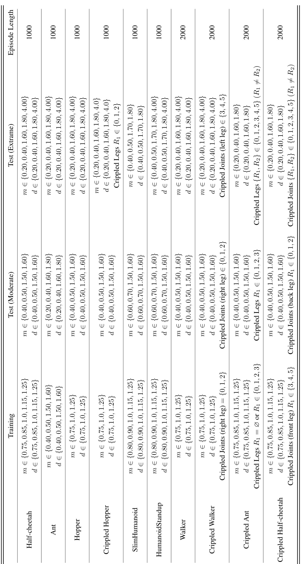
🔼 This table compares the average return and standard deviation achieved by different meta-reinforcement learning algorithms (PEARL, TESAC, CCM, SaTESAC, and SaCCM) across various MuJoCo tasks. The tasks are categorized into training, moderate test, and extreme test sets, reflecting the difficulty and generalization capabilities of the algorithms. The asterisk (*) indicates statistically significant improvement (p<0.05) of the SaMI-based algorithms (SaTESAC and SaCCM) compared to their non-SaMI counterparts (TESAC and CCM). Bold numbers highlight the best-performing algorithm for each task category.
read the caption
Table 2: Comparison of average return ± standard deviation with baselines in modified MuJoCo benchmark (over 5 seeds). Bold number signifies the highest return. * next to the number means that the algorithm with SaMI has statistically significant improvement over the same algorithm without SaMI. All significance claims based on t-tests with significance threshold of p < 0.05.
🔼 This table presents the comparison of success rates achieved by different meta-reinforcement learning algorithms on the Panda-gym benchmark. The algorithms are evaluated in three conditions: training, moderate testing, and extreme testing. The table highlights the statistically significant improvements achieved by algorithms incorporating the proposed SaMI (Skill-aware Mutual Information) optimization objective, showcasing its effectiveness in enhancing zero-shot generalization.
read the caption
Table 1: Comparison of success rate ± standard deviation with baselines in Panda-gym (over 5 seeds). Bold text signifies the highest average return. * next to the number means that the algorithm with SaMI has statistically significant improvement over the same algorithm without SaMI. All significance claims based on paired t-tests with significance threshold of p < 0.05.

🔼 This table compares the average return and standard deviation of different reinforcement learning algorithms on the modified MuJoCo benchmark. It includes training and testing results (moderate and extreme difficulty levels), and highlights statistically significant improvements achieved by algorithms incorporating SaMI (Skill-aware Mutual Information). The results are averaged across five different random seeds, to provide a robust comparison. The bold values represent the highest average return for each setting.
read the caption
Table 2: Comparison of average return ± standard deviation with baselines in modified MuJoCo benchmark (over 5 seeds). Bold number signifies the highest return. * next to the number means that the algorithm with SaMI has statistically significant improvement over the same algorithm without SaMI. All significance claims based on t-tests with significance threshold of p < 0.05.

🔼 This table presents the average return and standard deviation achieved by different meta-reinforcement learning algorithms across various MuJoCo robotic control tasks. It compares the performance of algorithms with and without SaMI (Skill-aware Mutual Information), which is a novel optimization objective proposed in the paper. The results are presented for training tasks and separate test tasks of moderate and extreme difficulty. The table highlights statistically significant improvements achieved by algorithms incorporating SaMI.
read the caption
Table 2: Comparison of average return ± standard deviation with baselines in modified MuJoCo benchmark (over 5 seeds). Bold number signifies the highest return. * next to the number means that the algorithm with SaMI has statistically significant improvement over the same algorithm without SaMI. All significance claims based on t-tests with significance threshold of p < 0.05.

🔼 This table compares the success rate (with standard deviation) of different algorithms on a Panda-gym benchmark, specifically focusing on the impact of SaMI (Skill-aware Mutual Information) on zero-shot generalisation performance. It shows the success rates in training and testing environments with moderate and extreme difficulty levels. Statistical significance of improvements by SaMI over baselines is also indicated.
read the caption
Table 1: Comparison of success rate ± standard deviation with baselines in Panda-gym (over 5 seeds). Bold text signifies the highest average return. * next to the number means that the algorithm with SaMI has statistically significant improvement over the same algorithm without SaMI. All significance claims based on paried t-tests with significance threshold of p < 0.05.

🔼 This table presents the p-values obtained from paired t-tests comparing the performance of algorithms with and without SaMI in the Panda-gym benchmark. A p-value less than 0.05 indicates a statistically significant improvement due to the inclusion of SaMI. The table shows the p-values for training, moderate testing, and extreme testing scenarios for both SaTESAC (compared to TESAC) and SaCCM (compared to CCM).
read the caption
Table 8: The p-value of the statistical hypothesis tests (paried t-tests) for comparing the effectiveness of SaMI in Panda-gym benchmark (over 5 seeds). * next to the number means that the algorithm with SaMI has statistically significant improvement over the same algorithm without SaMI at a significance level of 0.05. The “SaTESAC-TESAC” row indicates the p-value for the return improvement brought by SaMI to TESAC; the “SaCCM-CCM” row indicates the p-value for the return improvement brought by SaMI to CCM.
Full paper#
