TL;DR#
Solving parametric partial differential equations (PDEs) is critical in many fields, but existing machine learning methods struggle to generalize well across different PDE parameters due to limited data and the complexity of the underlying dynamics. Traditional approaches often require enormous datasets, which are often unavailable in practical applications. This leads to poor performance when the model is presented with new, unseen parameter configurations.
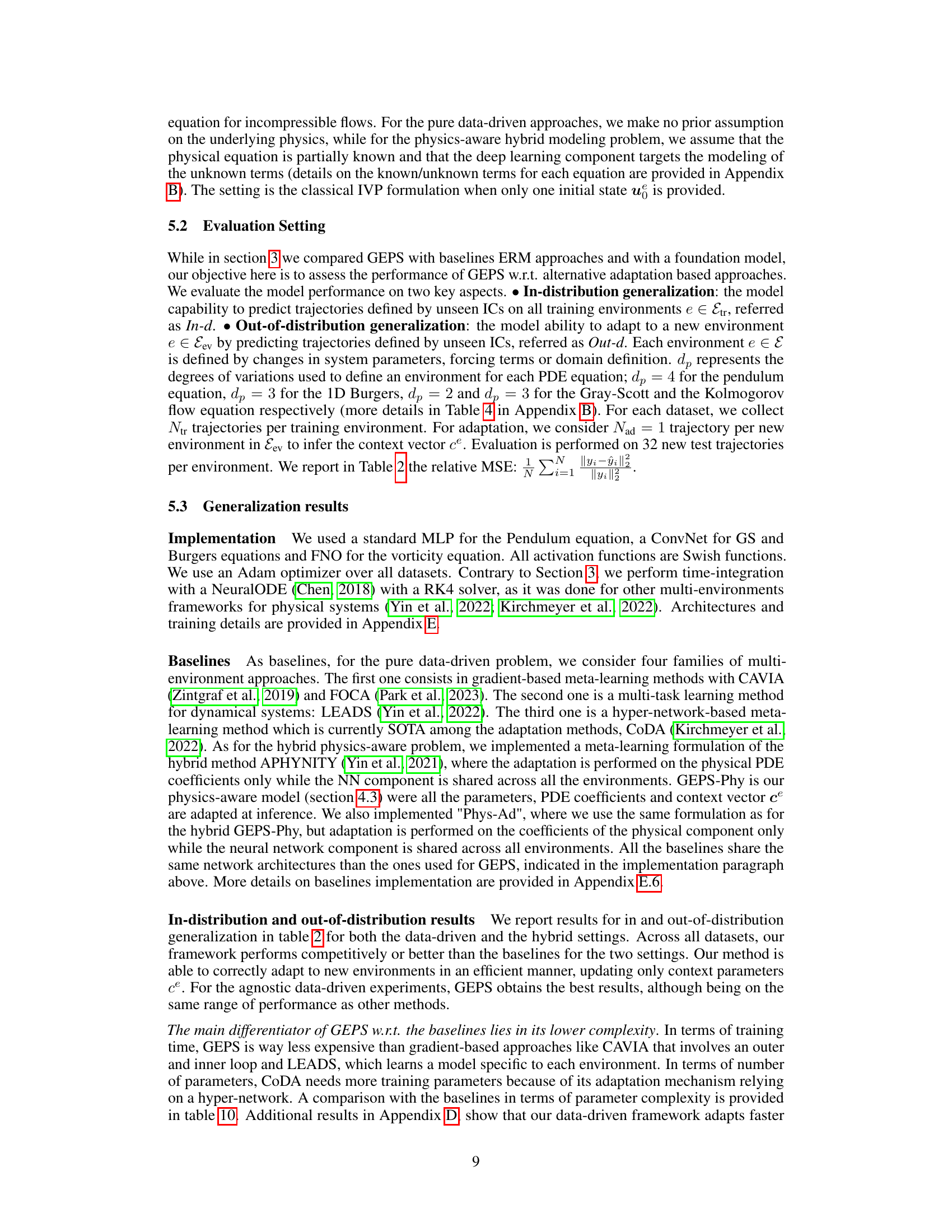
The paper introduces GEPS, a novel method that addresses these challenges by incorporating adaptive conditioning mechanisms. GEPS utilizes a first-order optimization technique with low-rank rapid adaptation, improving generalization without requiring extensive data. The method’s effectiveness is validated across various PDE problems and demonstrates strong performance compared to traditional techniques. GEPS is versatile and compatible with diverse neural network architectures, making it a valuable tool for a wide range of applications.
Key Takeaways#
Why does it matter?#
This paper is crucial for researchers working with parametric PDEs, particularly those facing generalization challenges with limited data. It offers a scalable and efficient solution for enhancing the performance of neural PDE solvers, opening new avenues for research in various scientific and engineering disciplines reliant on accurate PDE modeling.
Visual Insights#
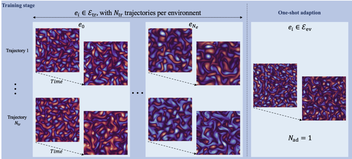
🔼 The figure illustrates the training and inference stages for solving parametric PDEs. The training stage involves multiple environments (each defined by unique parameters), with multiple trajectories sampled within each environment. The inference stage demonstrates the model’s ability to adapt to a single trajectory from a completely new, unseen environment.
read the caption
Figure 1: Multi-environment setup for the Kolmogorov PDE. The model is trained on multiple environments with several trajectories per environment (left). At inference, for a new unseen environment it is adapted on one trajectory (right).
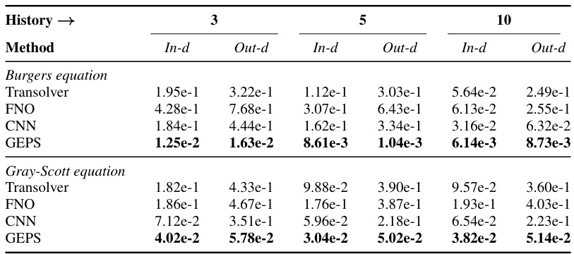
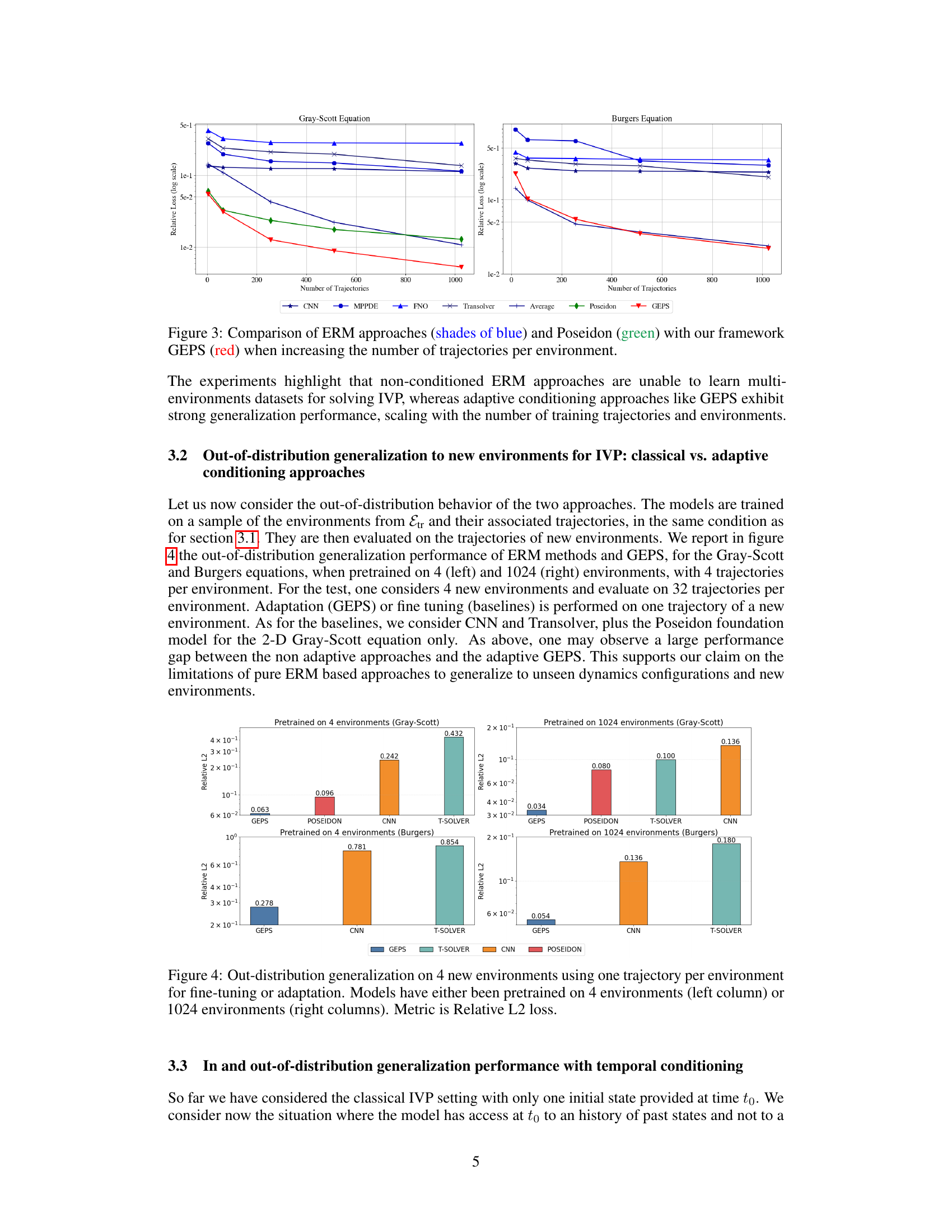
🔼 This table compares the in-distribution and out-of-distribution generalization performance of different methods (Transolver, FNO, CNN, and GEPS) for solving parametric PDEs (Burgers and Gray-Scott equations) using temporal conditioning. The ‘History’ column shows the number of past states used for conditioning (3, 5, or 10), while ‘In-d’ represents in-distribution performance and ‘Out-d’ represents out-of-distribution performance. Relative L2 loss is the performance metric.
read the caption
Table 1: In-distribution and out-distribution results comparing different history window sizes. Metric is the Relative L2 loss.
In-depth insights#
Adaptive Conditioning#
Adaptive conditioning, in the context of parametric partial differential equation (PDE) solvers, is a crucial technique for enhancing generalization. Traditional methods often struggle to generalize to unseen PDE parameters due to the complex interplay between parameters and spatiotemporal dynamics. Adaptive conditioning addresses this by dynamically adjusting the model’s behavior based on the specific parameters of a given PDE instance. This contrasts with standard approaches that rely on fixed model parameters across all instances. The core benefit is improved generalization to unseen conditions as the model learns to adapt rather than memorize specific parameter-solution pairings. Furthermore, adaptive conditioning facilitates more data-efficient training, as the model can generalize from fewer examples by learning to adapt. The choice of adaptation mechanism, its efficiency, and scalability with increasing numbers of parameters are key considerations in designing effective adaptive conditioning strategies. The paper explores various adaptive conditioning methods and emphasizes its practical implications for building robust and versatile parametric PDE solvers.
GEPS Framework#
The GEPS framework introduces a novel adaptive conditioning mechanism for training neural PDE solvers. Its core innovation is a first-order, low-rank adaptation technique, allowing for efficient generalization to unseen environments defined by varying parameters. This approach contrasts with traditional methods that struggle to handle the high dimensionality and sensitivity of PDEs. GEPS’s low-rank adaptation is particularly efficient, requiring only a small number of context parameters to adapt to new environments. The framework demonstrates compatibility with various neural network architectures, accommodating both data-driven and physics-aware solvers. Its effectiveness is validated across a range of PDEs, showcasing robust out-of-distribution generalization while maintaining high in-distribution performance. A key advantage is its scalability, enabling efficient adaptation even in scenarios with limited data or numerous environments. The overall design suggests a promising approach for advancing the applicability of neural solvers to complex scientific and engineering problems.
Generalization Tests#
The effectiveness of a machine learning model hinges on its ability to generalize, and this is especially crucial in the context of parametric partial differential equations (PDEs). In this scenario, thorough generalization tests are paramount to gauge the model’s capacity to predict dynamics accurately under diverse conditions. Such tests could include in-distribution generalization, which assesses the model’s performance on unseen initial conditions or forcing terms while maintaining the same PDE coefficients, and out-of-distribution generalization, which evaluates its performance on different PDE parameters or even modified PDE structures. The results would be a quantitative assessment of the model’s robustness, and in the case of a failure, provide insights into limitations. Few-shot learning capabilities could also be tested, demonstrating the ability of the model to adapt to new environments with a minimal amount of data. The results of the generalization tests would be essential in determining the model’s applicability and reliability in practical scenarios. Careful evaluation of model performance across a spectrum of scenarios is critical to building trust in the methodology and revealing whether any assumptions made during the model design process were oversimplified.
Hybrid PDE Models#
Hybrid PDE models combine the strengths of data-driven methods and physics-based models to overcome limitations of each approach alone. Data-driven components, such as neural networks, learn complex, non-linear relationships from data, while physics-based components, often involving numerical solvers or established PDE formulations, ensure physical consistency and provide regularization. This synergy allows for improved accuracy and generalizability, particularly when dealing with incomplete or uncertain physical knowledge. The neural networks can learn residual terms or aspects of the system that are difficult to model analytically, augmenting the physics-based model for a more complete representation. However, effective design requires careful consideration of how to integrate the two components, balancing the need for flexibility and data efficiency from the neural network with the constraint of maintaining physically plausible solutions from the physics-based element. Key challenges include finding appropriate ways to encode and incorporate physical knowledge, determining how much data is needed to effectively train the neural network, and selecting suitable numerical schemes that are compatible with the data-driven learning process.
Future Directions#
Future research could explore enhanced generalization by investigating alternative adaptation mechanisms beyond the proposed low-rank approach, potentially leveraging more sophisticated meta-learning techniques or incorporating inductive biases from physics. Scalability to even larger, more complex PDEs and higher-dimensional spaces remains a key challenge, requiring investigation of efficient model architectures and training strategies. A crucial area for future work is handling uncertainty in PDE parameters and data, including developing robust methods for quantifying uncertainty in predictions. The impact of different numerical solvers on the efficacy of the proposed framework needs further exploration. Finally, a more thorough investigation into the applicability of the framework to real-world problems across diverse scientific and engineering domains is essential to showcase its practical value and identify potential limitations. Further work could also focus on the development of more intuitive and interpretable methods for understanding the adaptive conditioning mechanism’s behavior.
More visual insights#
More on figures

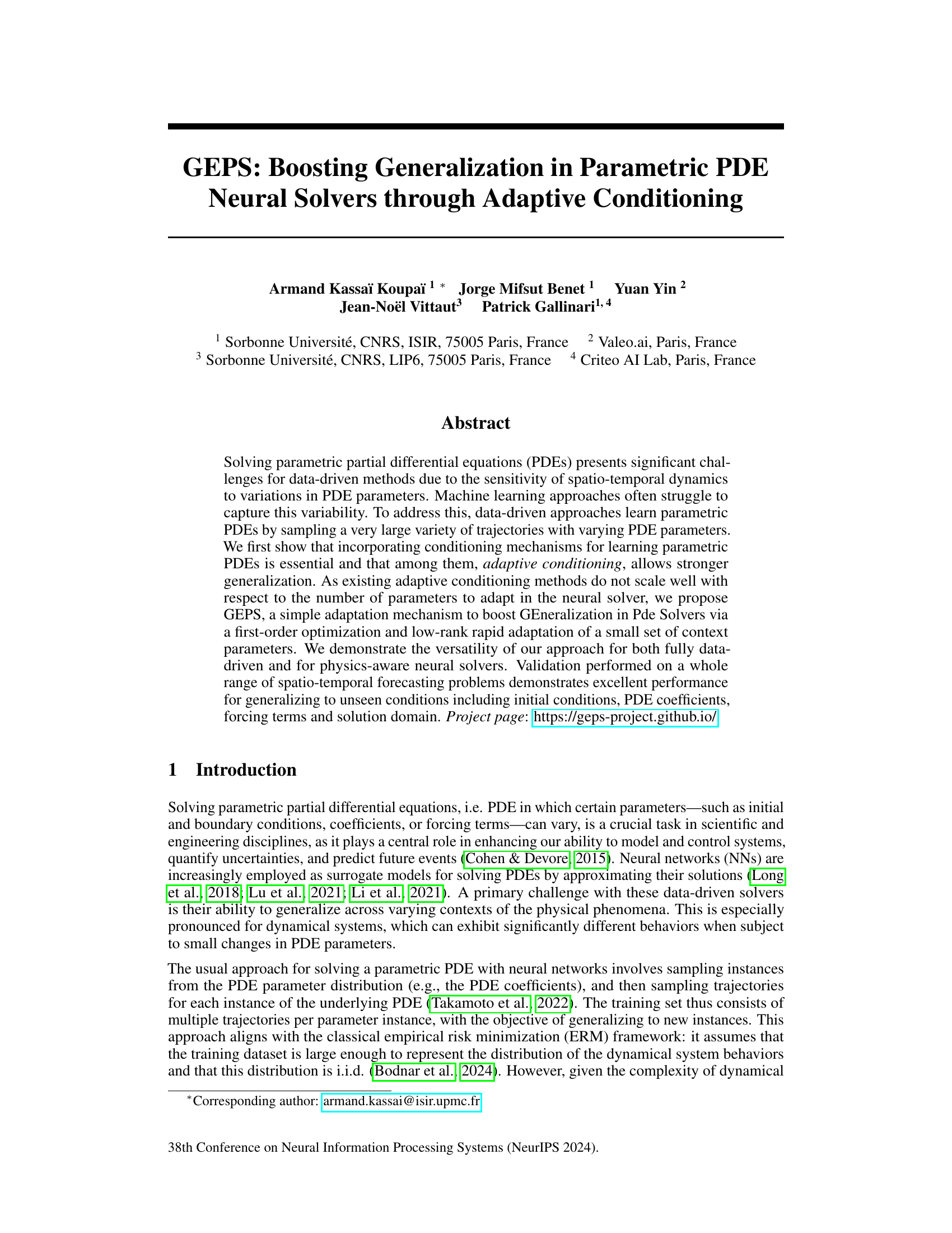
🔼 The figure compares the performance of several methods for solving parametric PDEs, including classical ERM approaches with different neural network architectures (CNN, FNO, MP-PDE, Transolver) and a pre-trained foundation model (Poseidon), against the proposed GEPS method. The experiment is performed for in-distribution generalization, where the number of training environments is varied. The results show that GEPS consistently outperforms other methods, especially as the number of training environments increases, highlighting the effectiveness of adaptive conditioning in handling the diversity of dynamical systems.
read the caption
Figure 2: Comparison of ERM approaches (shades of blue) and Poseidon foundation model (green) with our framework GEPS (red) when increasing the number of training environments.

🔼 The figure compares the performance of various neural PDE solvers, including ERM approaches (CNN, FNO, MP-PDE, Transolver) and a foundation model (Poseidon), against the proposed GEPS method, under in-distribution evaluation. The x-axis represents the number of training environments, and the y-axis represents the relative L2 loss on 32 unseen trajectories. The results show that ERM approaches fail to capture the dynamics of increasing environments while the GEPS method demonstrates superior generalization performance.
read the caption
Figure 2: Comparison of ERM approaches (shades of blue) and Poseidon foundation model (green) with our framework GEPS (red) when increasing the number of training environments.
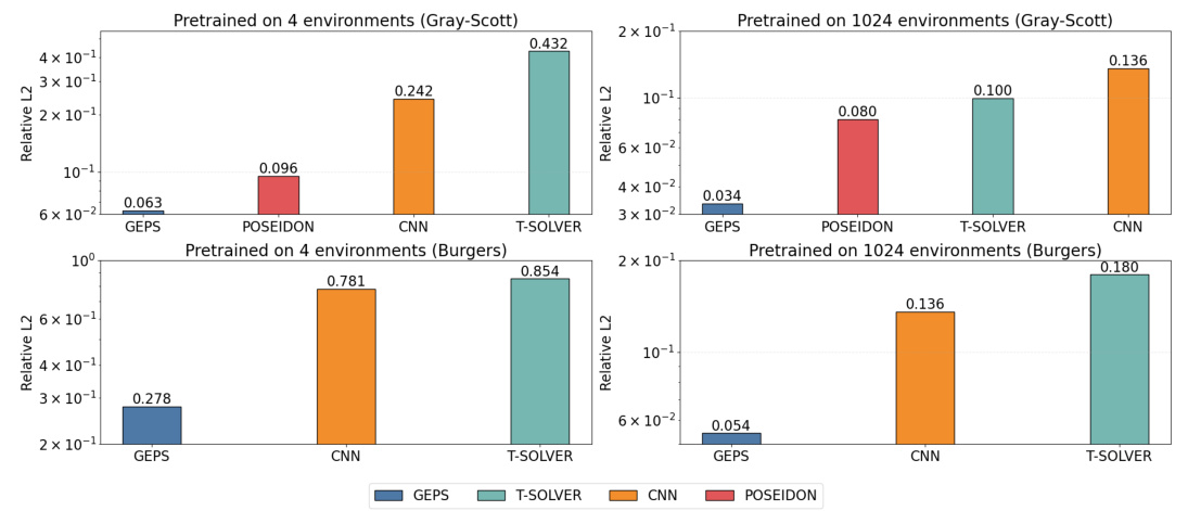
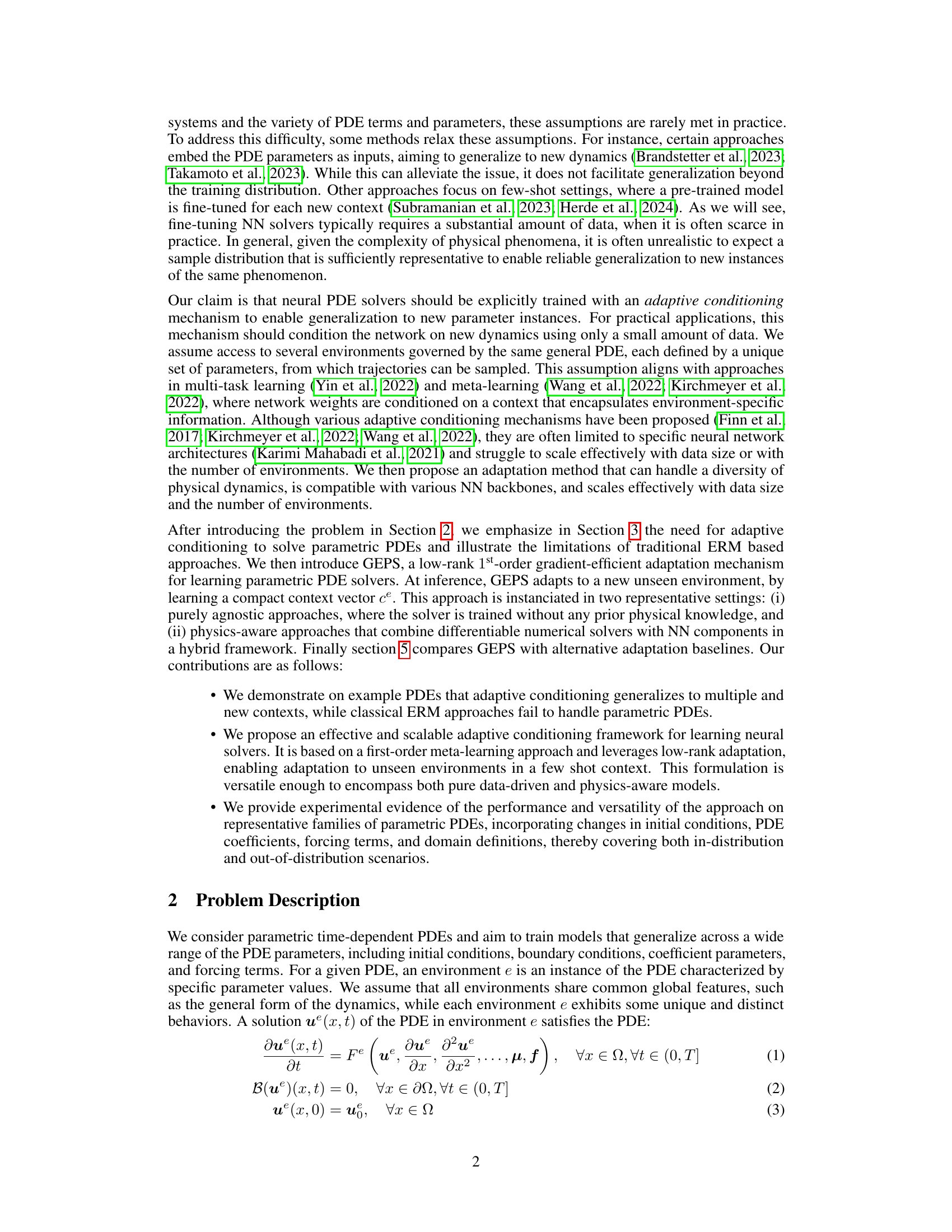
🔼 This figure compares the out-of-distribution generalization performance of different models (GEPS, CNN, Transolver, and Poseidon) when pretrained on either 4 or 1024 environments. The models are evaluated on 4 new environments, using only one trajectory from each for adaptation (or fine-tuning for the baselines). Relative L2 loss is shown for the Gray-Scott and Burgers equations, illustrating GEPS’s superior performance in out-of-distribution scenarios.
read the caption
Figure 4: Out-distribution generalization on 4 new environments using one trajectory per environment for fine-tuning or adaptation. Models have either been pretrained on 4 environments (left column) or 1024 environments (right columns). Metric is Relative L2 loss.
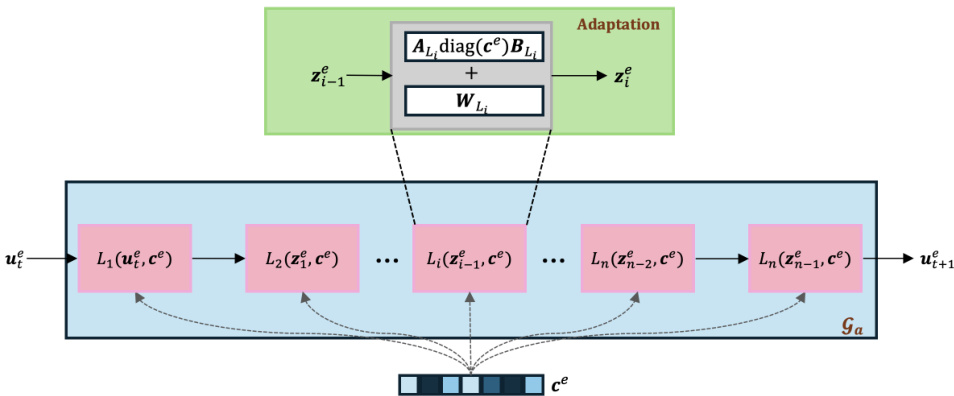
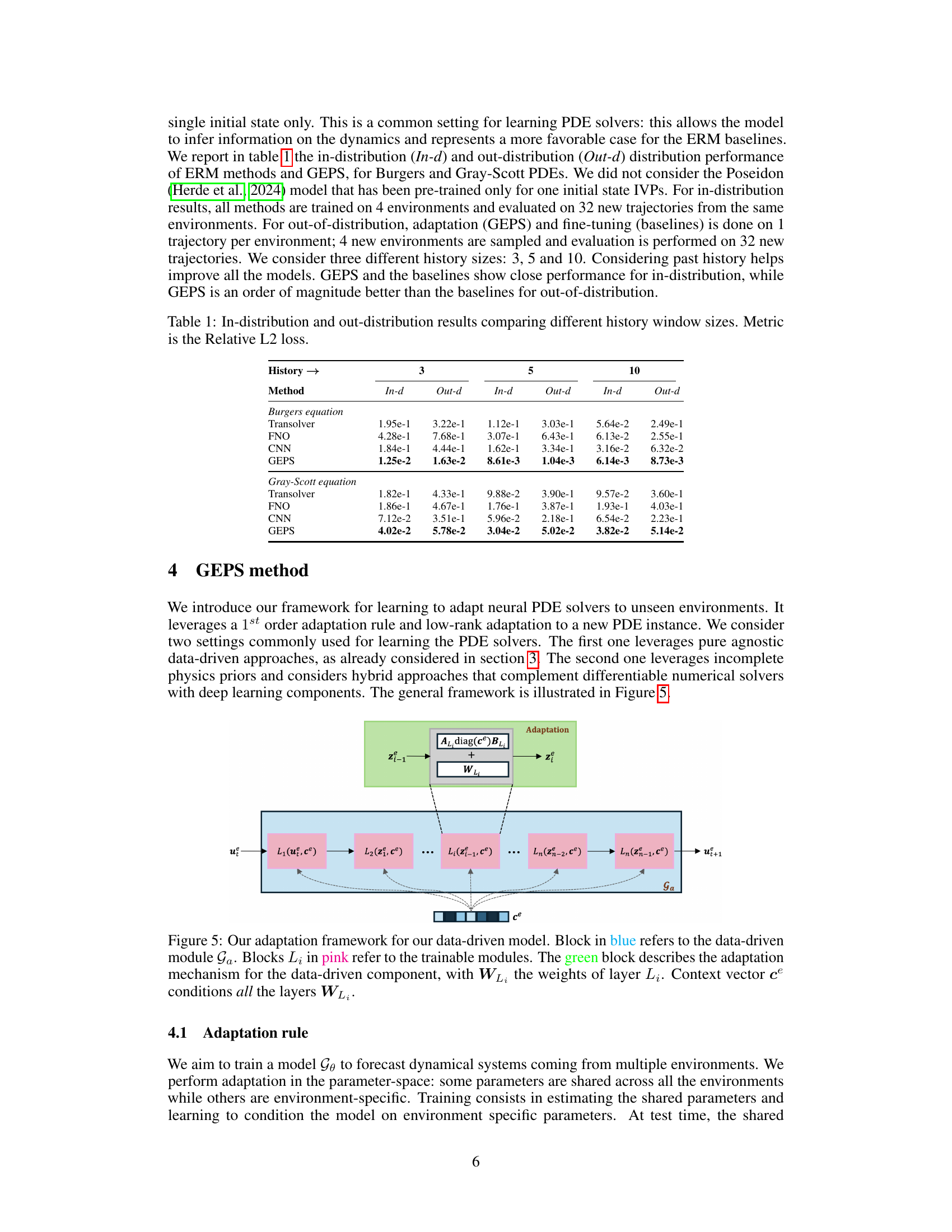
🔼 This figure illustrates the adaptation framework used in the GEPS method for data-driven models. It shows a series of trainable modules (pink blocks) forming the core of the data-driven model (Ga, blue block). A key element is the adaptive conditioning mechanism (green block) which updates a context vector (ce) to adapt to new unseen environments. This adaptation modifies the weights of each layer (Li) via a low-rank update using the context vector and pre-trained shared parameters (WL). The input (ue) is processed sequentially through the modules and the output (ue_t+1) represents the model’s prediction for the next time step.
read the caption
Figure 5: Our adaptation framework for our data-driven model. Block in blue refers to the data-driven module Ga. Blocks Li in pink refer to the trainable modules. The green block describes the adaptation mechanism for the data-driven component, with WL₁ the weights of layer Li. Context vector ce conditions all the layers WL₁.

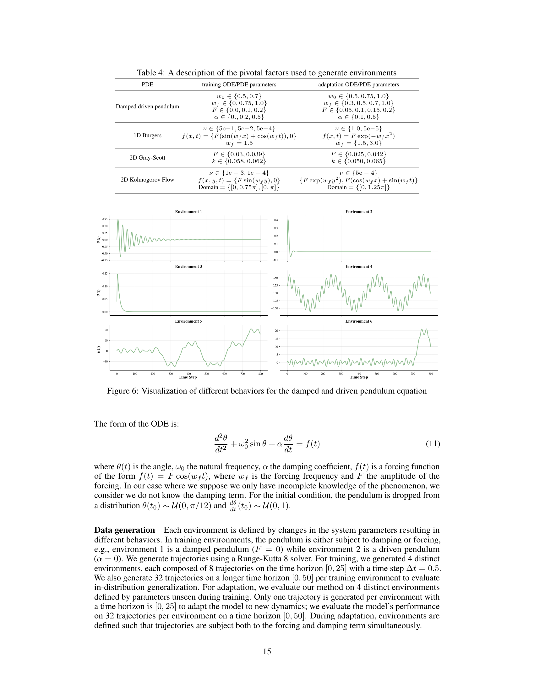
🔼 This figure visualizes six different behaviors of a damped and driven pendulum equation. Each environment represents a unique set of parameters resulting in distinct pendulum motions. The plots show the angle θ(t) over time, showcasing variations like underdamped oscillations, overdamped decay, resonance, and more complex behaviors under the influence of both damping and forcing terms. The figure is key to illustrating the diverse dynamics captured in the paper’s experiments, motivating the need for models capable of generalizing across these widely varying conditions.
read the caption
Figure 6: Visualization of different behaviors for the damped and driven pendulum equation

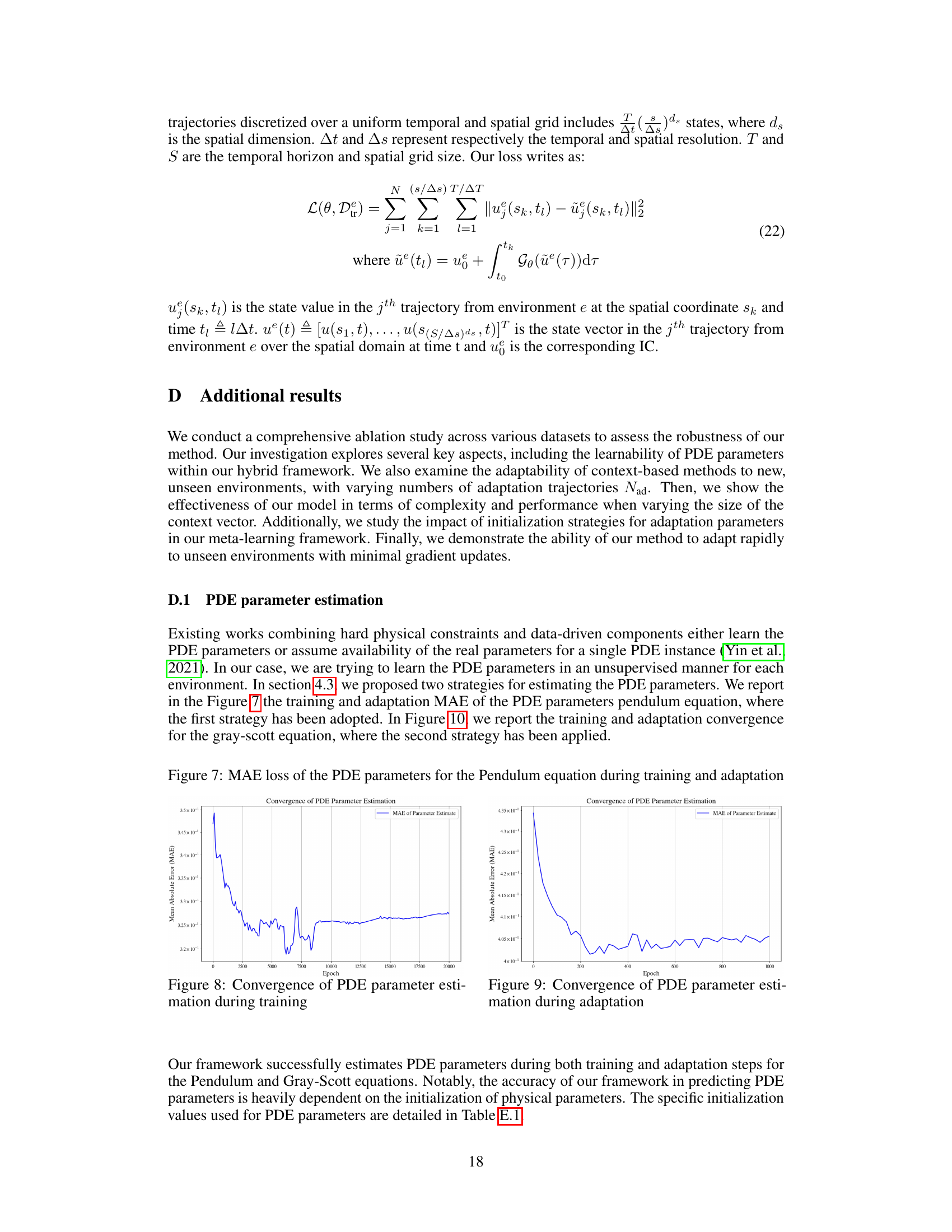
🔼 The figure shows the mean absolute error (MAE) loss for the PDE parameters of the pendulum equation during both the training and adaptation phases of the GEPS model. The training phase involves learning initial parameters across multiple environments. The adaptation phase focuses on updating parameters for a specific new environment. The plot illustrates how the MAE decreases over epochs (training iterations) during both training and adaptation, indicating that the model effectively learns and adapts the PDE parameters. The convergence behavior provides insights into the effectiveness of the proposed GEPS model in estimating and adapting PDE parameters for diverse scenarios.
read the caption
Figure 7: MAE loss of the PDE parameters for the Pendulum equation during training and adaptation

🔼 This figure shows the mean absolute error (MAE) loss during training and adaptation of the PDE parameters for the Pendulum equation. The plot displays the convergence of the MAE over epochs. The graph illustrates the effectiveness of the method for estimating PDE parameters both during the initial training phase and the subsequent adaptation phase when presented with new, unseen environments.
read the caption
Figure 7: MAE loss of the PDE parameters for the Pendulum equation during training and adaptation
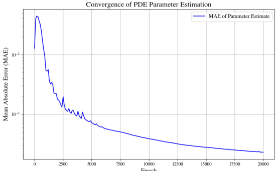
🔼 This figure shows the Mean Absolute Error (MAE) loss for the estimation of PDE parameters during both training and adaptation phases for the Pendulum equation. The plot displays the MAE over epochs, illustrating the convergence of the parameter estimation process during training and its rapid adaptation when presented with new unseen environments during the adaptation phase.
read the caption
Figure 7: MAE loss of the PDE parameters for the Pendulum equation during training and adaptation

🔼 This figure shows the mean absolute error (MAE) loss during the training and adaptation phases for estimating PDE parameters in the pendulum equation. It illustrates the convergence of the parameter estimation process over training epochs and during the adaptation to new, unseen environments.
read the caption
Figure 7: MAE loss of the PDE parameters for the Pendulum equation during training and adaptation
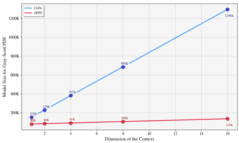
🔼 The figure shows how the model size changes with respect to the code dimension for both CoDa and GEPS on the Gray-Scott PDE. It demonstrates the impact of the context vector’s dimensionality on the overall number of parameters in each model. GEPS shows significantly smaller model sizes across different context dimensions compared to CoDa.
read the caption
Figure 13: Model size with respect to code dimension
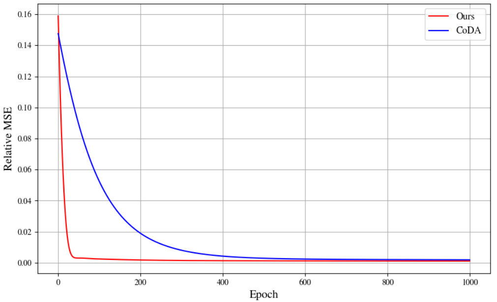
🔼 This figure compares the convergence speed of the proposed GEPS method and the CoDA method for adapting to new environments in the Burgers dataset. GEPS shows significantly faster convergence, reaching a stable state in under 100 epochs, while CoDA requires approximately 500 epochs. Both methods used the same learning rate (lr = 0.01). This illustrates GEPS’s efficiency in adapting to new contexts.
read the caption
Figure 14: Convergence speed of the model Gθ to adapt to new environments for the Burgers dataset. Less than 100 steps, compared to CoDA which needs 500 steps. For both runs, we used the same learning rate lr = 0.01.

🔼 This figure illustrates the GEPS adaptation framework. The framework consists of a data-driven module (blue) and trainable modules (pink). The adaptation mechanism (green) uses a low-rank approximation with a context vector (ce) to adapt to new environments. The context vector conditions all the layers of the trainable modules, enabling efficient adaptation with minimal parameter updates.
read the caption
Figure 5: Our adaptation framework for our data-driven model. Block in blue refers to the data-driven module Ga. Blocks Li in pink refer to the trainable modules. The green block describes the adaptation mechanism for the data-driven component, with WL₁ the weights of layer Li. Context vector ce conditions all the layers WL₁.

🔼 This figure compares the performance of different models (Ground truth, GEPS, CoDA, CAVIA, and LEADS) in predicting a trajectory for the 1D Burgers equation. It shows both in-distribution (left) and out-of-distribution (right) generalization. The in-distribution results show how well the models predict trajectories with initial conditions from the training data distribution. The out-of-distribution results show how well the models generalize to initial conditions outside of the training data distribution. Each row represents a different model, and each column represents a different time step. The color gradient represents the amplitude of the predicted trajectory, going from purple (low amplitude) to red (high amplitude).
read the caption
Figure 16: Comparison of in-distribution and out-distribution predictions of a trajectory on 1D Burgers. The trajectories are predicted from t = 0 (purple) to t = 0.1 (red).
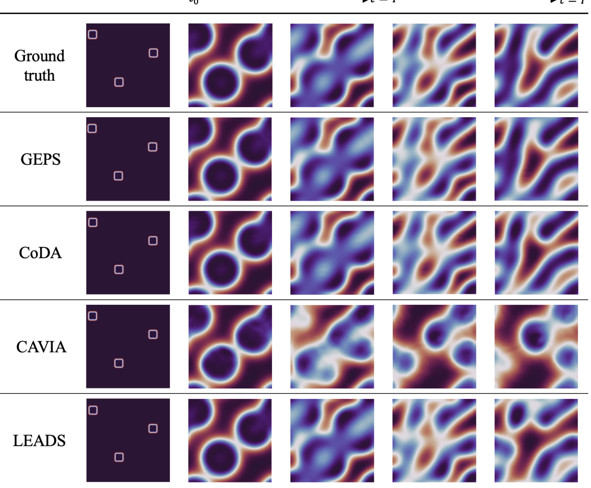
🔼 This figure compares the performance of different models in predicting the evolution of a 2D Gray-Scott system. The ‘Ground truth’ shows the actual evolution of the system. The other rows show the predictions by various models (GEPS, CoDA, CAVIA, LEADS) for an out-of-distribution trajectory (meaning the model was not trained on this specific parameter set). The figure illustrates how well each model generalizes to unseen conditions. It is organized to show the initial conditions and predictions at different time steps (t=0 to t=T’, where T=19 and T’=39).
read the caption
Figure 17: Prediction per frame for our approach on 2D Gray-Scott for an out-of-distribution trajectory. The trajectory is predicted from t = 0 to t = T'. In our setting, T = 19 and T' = 39.
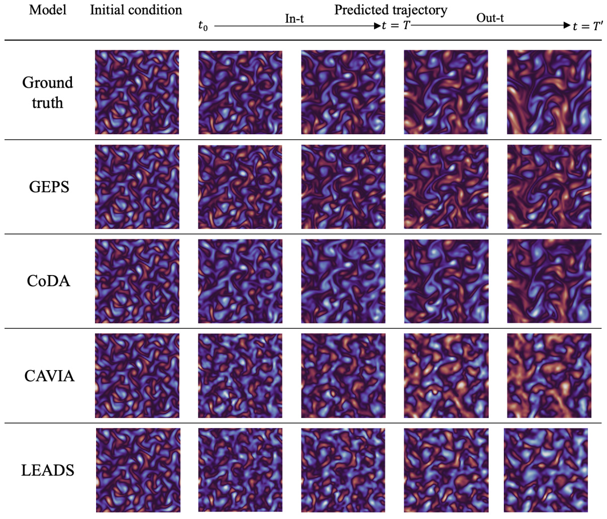
🔼 This figure compares the model’s predictions (GEPS, CoDA, CAVIA, LEADS) against the ground truth for a 2D Gray-Scott equation. It shows the model’s performance on an unseen (out-of-distribution) trajectory, demonstrating its ability to generalize to new conditions. The predictions are shown at different timesteps (t=0, t=T, and t=T’) illustrating the evolution of the system.
read the caption
Figure 17: Prediction per frame for our approach on 2D Gray-Scott for an out-of-distribution trajectory. The trajectory is predicted from t = 0 to t = T'. In our setting, T = 19 and T' = 39.
More on tables

🔼 This table presents the in-distribution and out-of-distribution generalization performance of various methods (LEADS, CAVIA, FOCA, CODA, GEPS, APHYNITY, Phys-Ad, GEPS-Phy) across four datasets (Pendulum, Gray-Scott, Burgers, Kolmogorov). The metrics used are the relative L2 loss for in-distribution and out-of-distribution generalization, with models fine-tuned using one trajectory per environment in the out-of-distribution setting. A ‘-’ indicates divergence during inference.
read the caption
Table 2: In-distribution and Out-of-distribution results on 32 new test trajectories per environment. For out-of-distribution generalization, models are fine-tuned on 1 trajectory per environment. Metric is the relative L2 loss. '-' indicates inference has diverged.
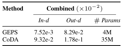
🔼 This table presents the in-distribution and out-of-distribution generalization performance of GEPS and CoDA models on a larger dataset with a larger model. The in-distribution results evaluate the model’s ability to generalize to unseen initial conditions within the training environments, while out-of-distribution results assess its ability to adapt to entirely new environments with limited data. The relative L2 loss metric measures the prediction error. The table also shows the number of parameters for each model, highlighting GEPS’s parameter efficiency.
read the caption
Table 3: In-distribution and Out-distribution results. Metric is the relative L2.
🔼 This table presents the in-distribution and out-of-distribution generalization results of different methods on four dynamical systems (Pendulum, Gray-Scott, Burgers, Kolmogorov). For out-of-distribution, the models are fine-tuned on only one trajectory per new environment. The results are evaluated using the relative L2 loss, and a ‘-’ indicates that the inference diverged.
read the caption
Table 2: In-distribution and Out-of-distribution results on 32 new test trajectories per environment. For out-of-distribution generalization, models are fine-tuned on 1 trajectory per environment. Metric is the relative L2 loss. '-' indicates inference has diverged.

🔼 This table presents the results of an experiment to evaluate the impact of the number of adaptation trajectories on the performance of three different models (CODA, CAVIA, and GEPS) when adapting context vectors. The results are reported as the Relative MSE loss for different numbers of adaptation trajectories (1, 4, 8, and 16).
read the caption
Table 5: Relative MSE loss with respect to number of adaptation trajectories when adapting context vectors ce.

🔼 This table shows the results of an experiment to evaluate the impact of the number of adaptation trajectories on the performance of the GEPS model when using low-rank adaptation of parameters. The experiment was conducted on the Kolmogorov flow equation. The Relative Mean Squared Error (MSE) is reported for different numbers of adaptation trajectories (1, 4, 8, and 16). The results show that reducing the number of adaptation trajectories improves the model’s performance.
read the caption
Table 6: Relative MSE loss with respect to number of adaptation trajectories when adapting low-rank adaptation parameters.
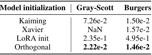
🔼 This table presents the relative Mean Squared Error (MSE) loss for different parameter initialization methods (Kaiming, Xavier, LoRA init, and Orthogonal) applied to the Gray-Scott and Burgers equations. The results show that orthogonal initialization achieves the lowest loss for both equations, indicating its superior performance in this context.
read the caption
Table 7: Relative MSE loss with respect to parameter initialization
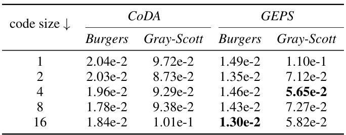
🔼 This table shows the performance of both CoDA and GEPS models on Burgers and Gray-Scott equations by varying the code dimension. It demonstrates the impact of code dimension on model performance, comparing the relative mean squared error (MSE) achieved by each method. The results highlight the trade-off between code size and model accuracy. A smaller code size may lead to faster adaptation but could sacrifice prediction accuracy.
read the caption
Table 8: Relative MSE on the full trajectory with varying code dimension

🔼 This table presents the in-distribution and out-of-distribution generalization performance of various models on four different datasets (Pendulum, Gray-Scott, Burgers, and Kolmogorov). In-distribution results assess the model’s ability to predict trajectories with unseen initial conditions within the same training environments. Out-of-distribution results evaluate the model’s ability to adapt to completely new environments (different PDE parameters) using only one trajectory for fine-tuning. The metric used is the relative L2 loss, and ‘-’ indicates that the inference process for that model and environment diverged.
read the caption
Table 2: In-distribution and Out-of-distribution results on 32 new test trajectories per environment. For out-of-distribution generalization, models are fine-tuned on 1 trajectory per environment. Metric is the relative L2 loss. '-' indicates inference has diverged.

🔼 This table presents a comparison of the number of parameters and training time required for different adaptive conditioning methods (LEADS, CAVIA, CODA, and GEPS) across four different dynamical systems (Pendulum, Gray-Scott, Burgers, and Kolmogorov). It highlights the computational efficiency of GEPS compared to other methods, particularly noticeable in the larger datasets.
read the caption
Table 10: Number of parameters (# Params) and training time (Time) for all different adaptive conditioning methods.

🔼 This table presents the in-distribution and out-of-distribution generalization performance of different models on the Burgers and Gray-Scott PDEs when using different history window sizes (3, 5, and 10). The relative L2 loss is used as the performance metric. The results demonstrate the performance of classical ERM (Empirical Risk Minimization) approaches compared to the adaptive conditioning approach (GEPS). The in-distribution results show performance on unseen trajectories from the training environments; out-of-distribution results show performance on unseen trajectories and environments.
read the caption
Table 1: In-distribution and out-distribution results comparing different history window sizes. Metric is the Relative L2 loss.
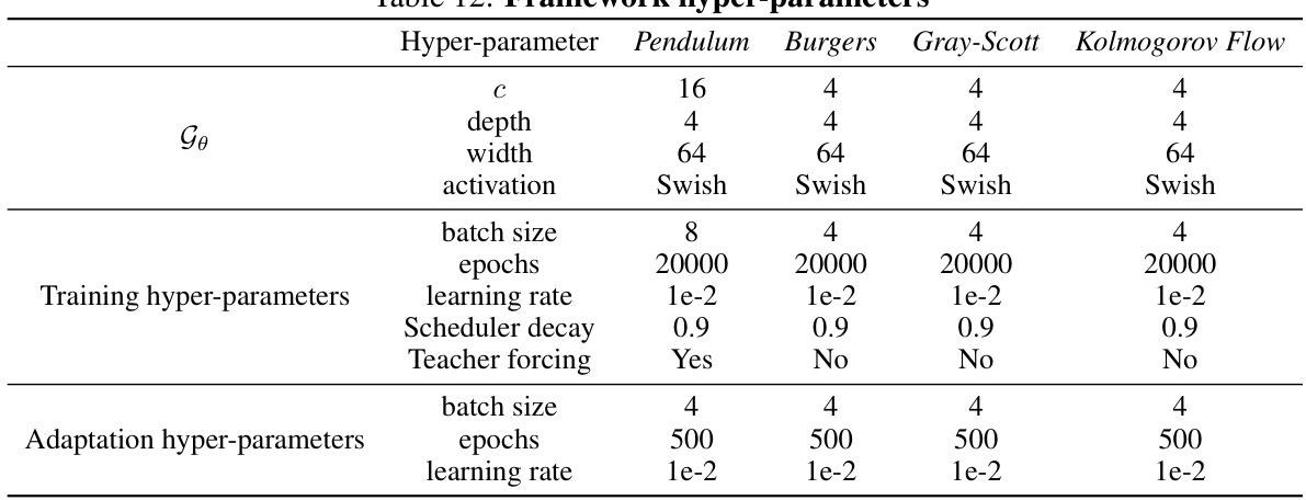
🔼 This table lists the hyperparameters used for training and adaptation for each of the four dynamical systems considered in the paper: Pendulum, Burgers, Gray-Scott, and Kolmogorov Flow. For each system, the table specifies the context size (c), network depth, width, activation function, batch size for training and adaptation, number of epochs for training and adaptation, and the learning rate used for both training and adaptation. Additionally, it indicates whether teacher forcing was used during training.
read the caption
Table 12: Framework hyper-parameters
Full paper#
