TL;DR#
Independent Component Analysis (ICA) is a powerful technique for separating mixed signals, but choosing the right algorithm is crucial, especially when dealing with noisy data. Existing methods often have limitations, struggling with different noise distributions and source characteristics. This research addresses these issues by focusing on a robust way to pick the best algorithm for a specific dataset.
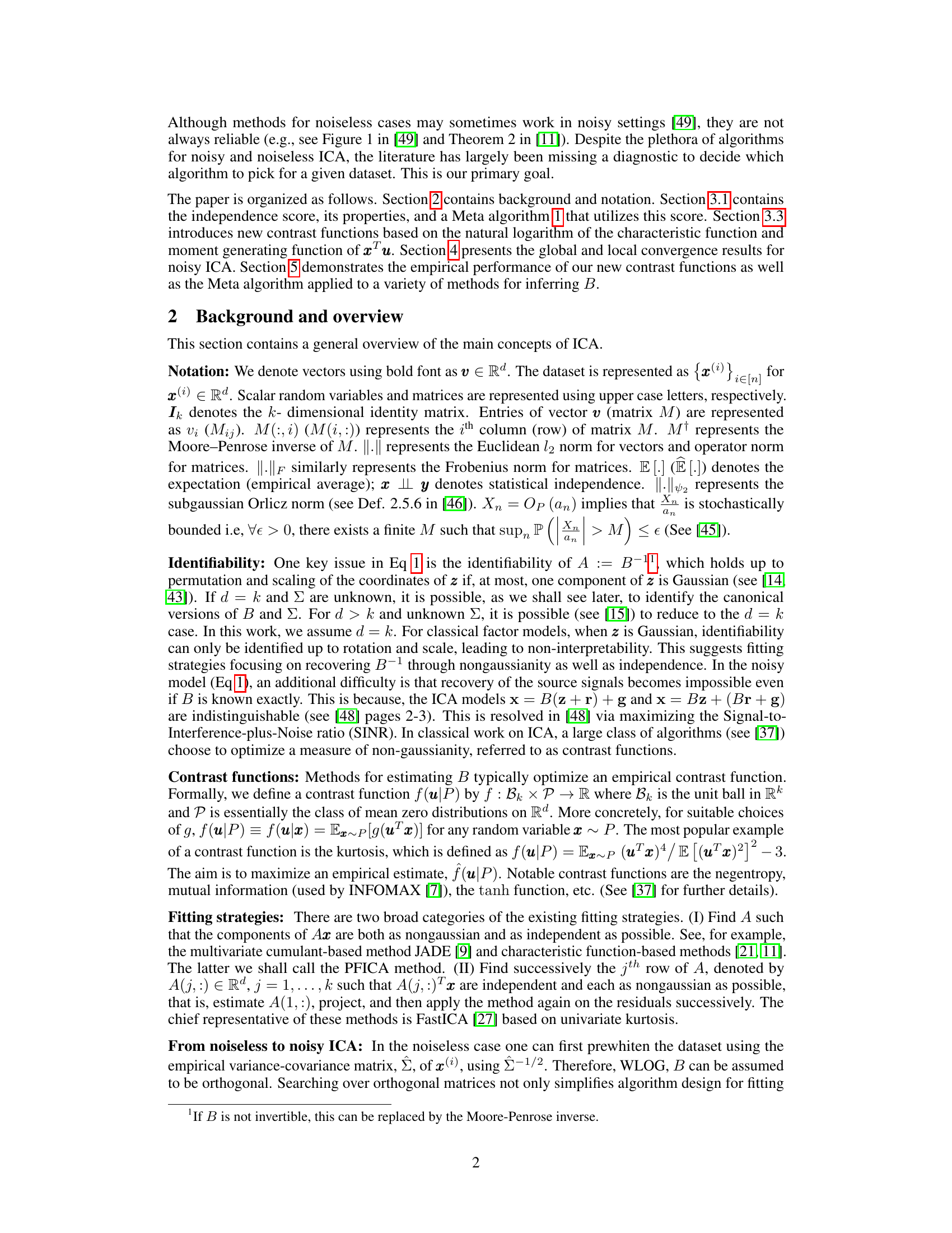
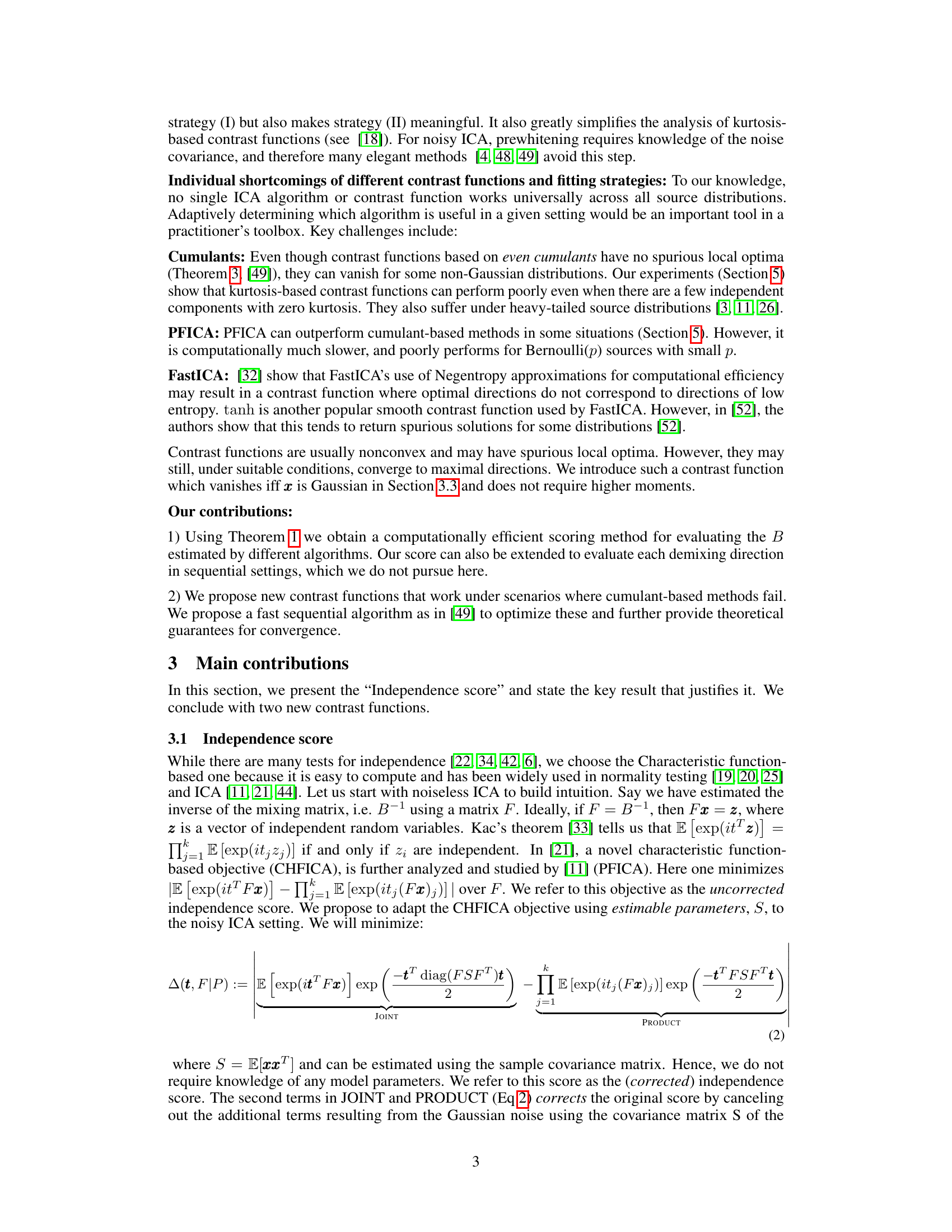
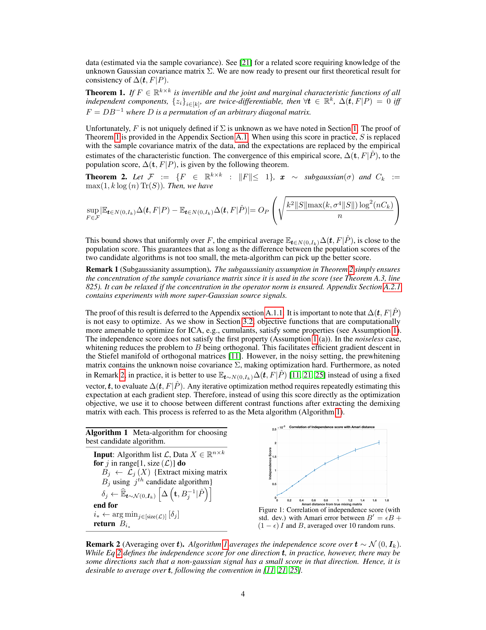
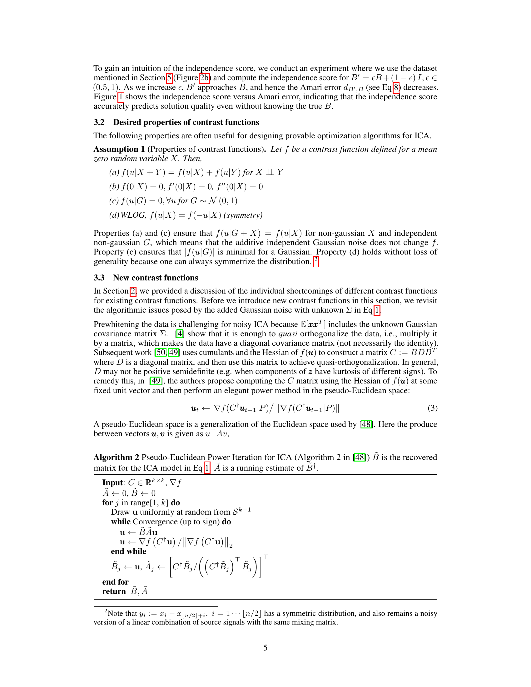
The core contribution is a novel non-parametric independence score. This score uses the characteristic function to evaluate the performance of different ICA algorithms, requiring only a finite second moment and not needing any parameters of the noise distribution. The study introduces two new contrast functions and proves their convergence, improving computational efficiency. A meta-algorithm then uses the independence score to select the best algorithm among the candidates, leading to higher accuracy in separating the signals.
Key Takeaways#
Why does it matter?#
This paper is crucial because it offers a novel solution to a long-standing challenge in Independent Component Analysis (ICA): selecting the optimal algorithm for noisy data. It introduces a non-parametric independence score to objectively evaluate ICA algorithms, allowing researchers to choose the best method for their specific dataset, regardless of noise distribution. This significantly advances ICA applications and related fields.
Visual Insights#

🔼 The figure shows the correlation between the independence score and the Amari distance from the true mixing matrix B. The independence score is a measure of how well the estimated mixing matrix (B’) approximates the true matrix B. The Amari distance is a commonly used metric for evaluating the performance of ICA algorithms. The plot demonstrates a strong positive correlation between the two metrics, indicating that a lower independence score corresponds to a smaller Amari distance (better performance). The error bars represent the standard deviation of the independence score across 10 random runs. This suggests the independence score can reliably predict the quality of ICA solutions.
read the caption
Figure 1: Correlation of independence score (with std. dev.) with Amari error between B' = єB + (1 - є) I and B, averaged over 10 random runs.

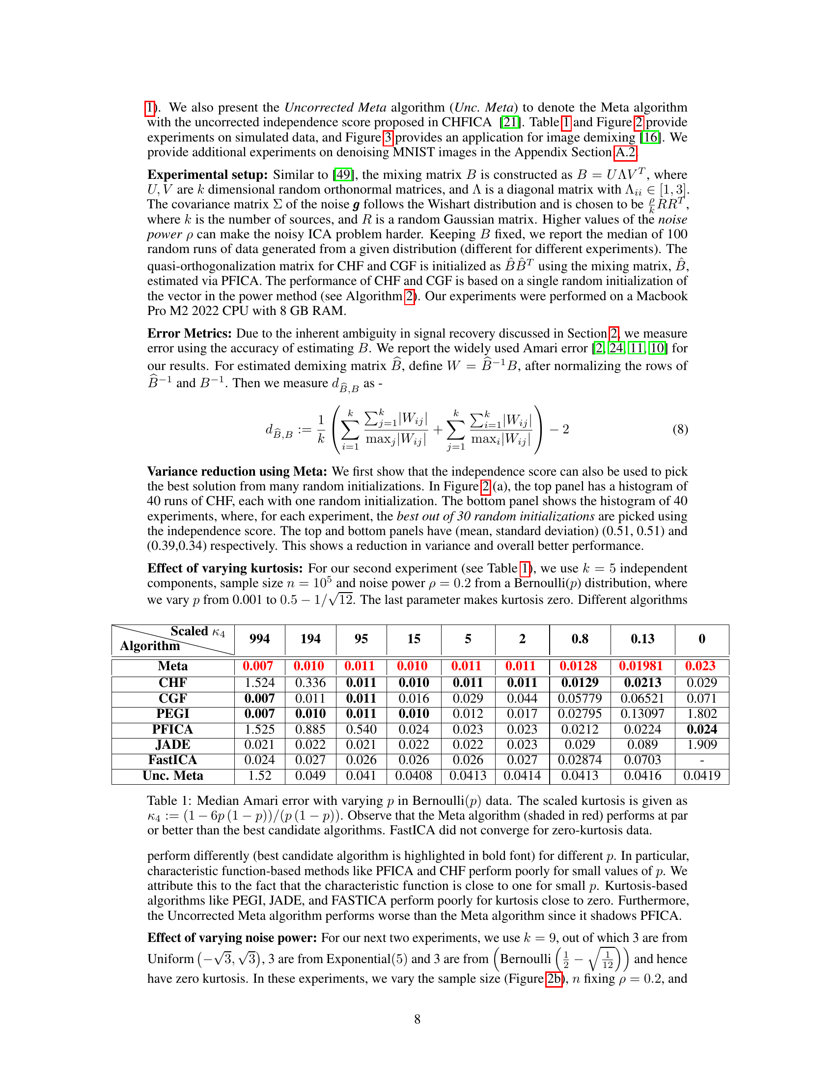
🔼 The table shows the median Amari error for different Bernoulli(p) distributions, varying the parameter p from 0.001 to 0.5. It compares the performance of several ICA algorithms (Meta, CHF, CGF, PEGI, PFICA, JADE, FastICA, and Unc. Meta), highlighting the effectiveness of the proposed Meta algorithm in selecting the best-performing algorithm for each value of p. The scaled kurtosis is also provided to show the relationship between kurtosis and algorithm performance.
read the caption
Table 1: Median Amari error with varying p in Bernoulli(p) data. The scaled kurtosis is given as К4 := (1 – 6p(1 − p))/(p(1 − p)). Observe that the Meta algorithm (shaded in red) performs at par or better than the best candidate algorithms. FastICA did not converge for zero-kurtosis data.
In-depth insights#
Noisy ICA Scope#
The scope of noisy independent component analysis (ICA) encompasses scenarios where observed signals are corrupted by additive Gaussian noise, a common real-world condition. Addressing this noise is crucial, as standard ICA methods designed for noiseless data often fail in such conditions. The challenge lies in disentangling the underlying sources from the noise, demanding robust algorithms and theoretical analysis. A key aspect of the noisy ICA scope is identifiability, which is the ability to uniquely recover the sources from the noisy mixture. This identifiability is often constrained by the unknown characteristics of the noise and the limited knowledge of the source distributions. The scope also involves developing efficient algorithms that can accurately estimate the mixing matrix and source signals in the presence of the noise, with guarantees of convergence. Finally, a comprehensive approach to noisy ICA involves establishing performance evaluation metrics, including statistical significance tests that account for the presence of noise, facilitating reliable comparisons among different algorithms and settings.
Independence Score#
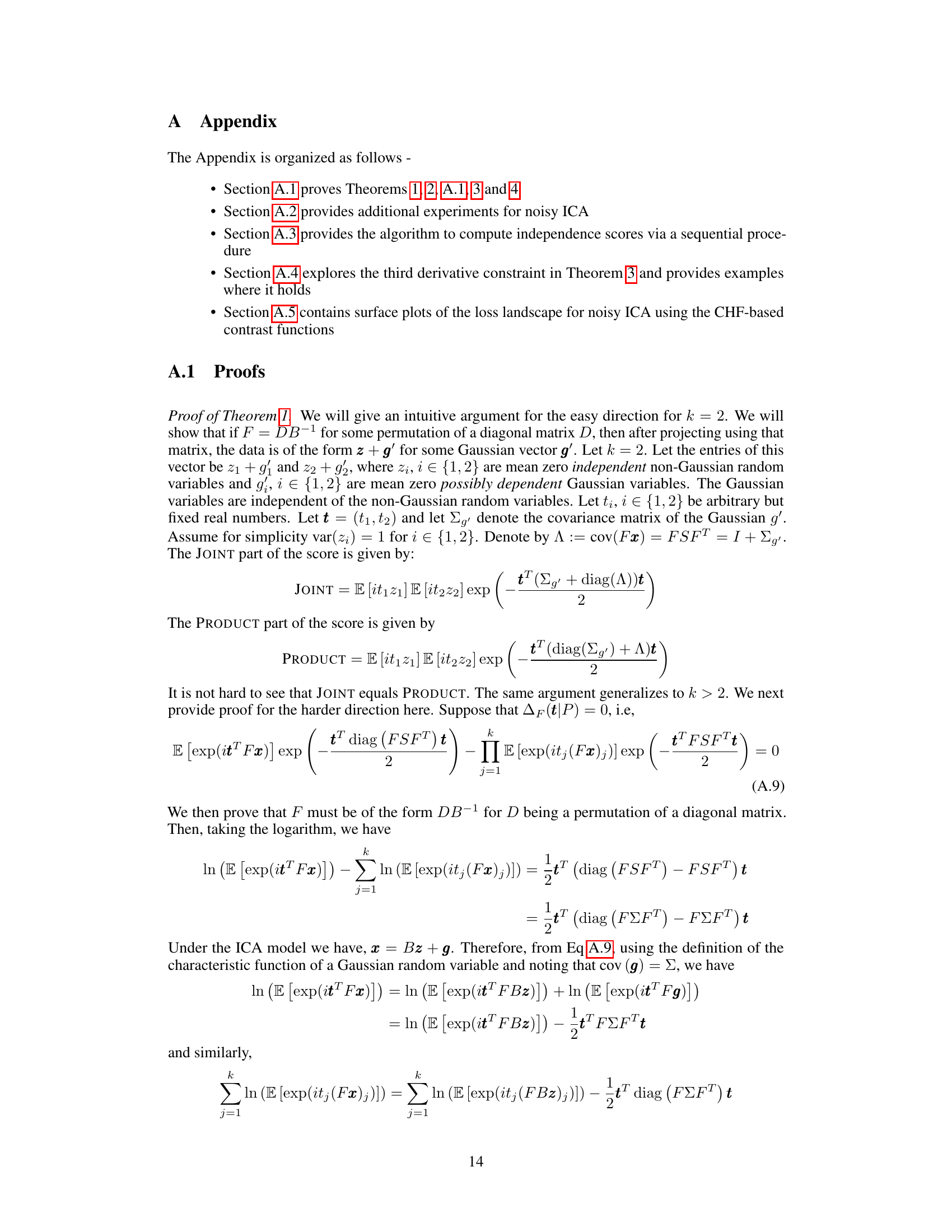
The concept of an ‘Independence Score’ in the context of noisy Independent Component Analysis (ICA) is a novel approach to evaluating the quality of ICA solutions. It leverages the characteristic function, a tool from probability theory, to assess the independence of estimated source signals without requiring knowledge of the noise distribution’s parameters or making assumptions about the source signals’ distributions beyond a finite second moment. This is crucial because real-world data often deviates from idealized assumptions, and the proposed method exhibits robustness. A key advantage is the method’s adaptability as it allows for the selection of the optimal algorithm among several candidates based on the independence score for a given dataset. The theoretical framework establishing its consistency and convergence properties, especially in the presence of noise, further enhances its value, contributing to more reliable and adaptable ICA solutions. The simulations demonstrate that this approach can identify and improve the performance of certain ICA algorithms and its ability to detect the optimal algorithm for a variety of scenarios further solidifies the importance of the Independence Score.
Contrast Functions#
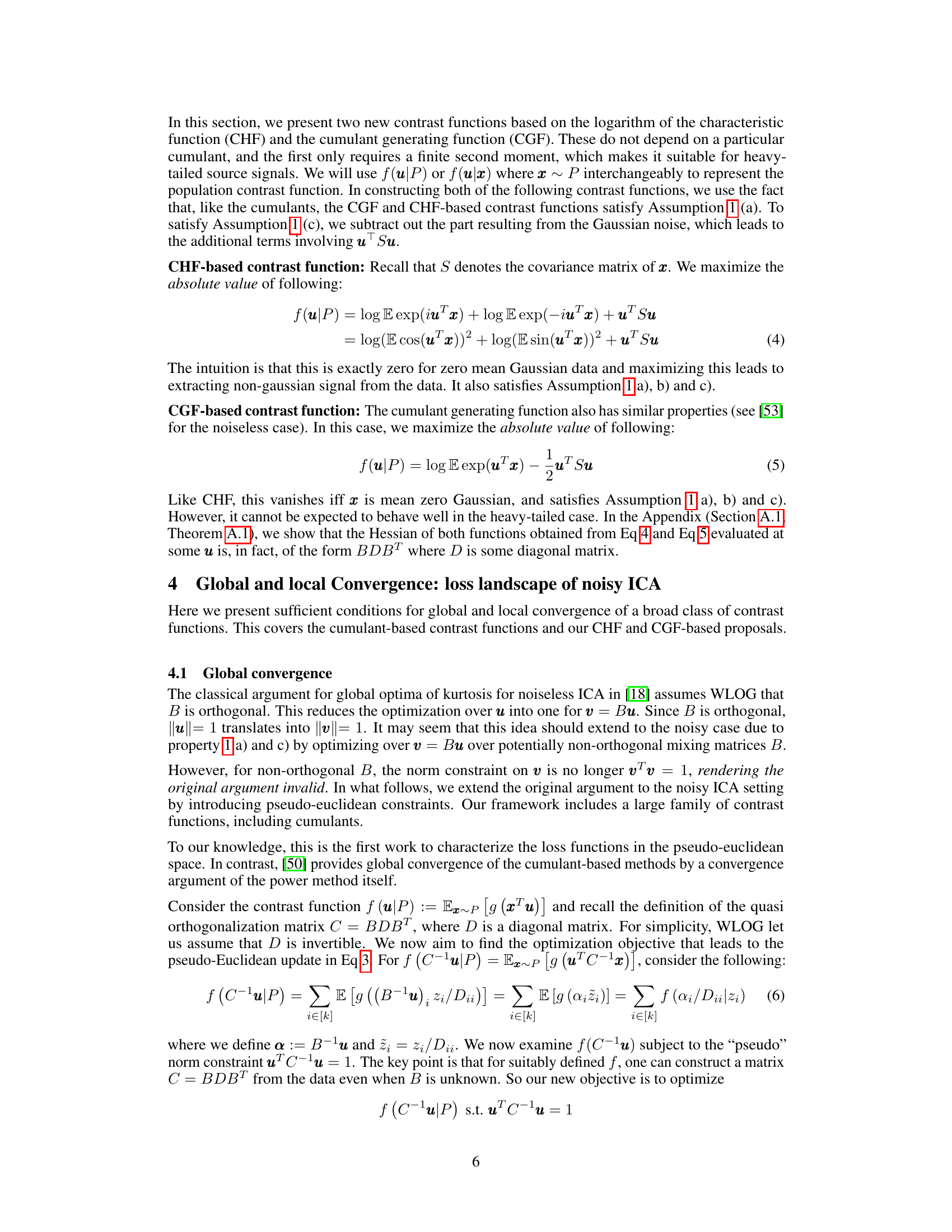
Contrast functions are core components in Independent Component Analysis (ICA), aiming to measure the non-Gaussianity of data. Their effectiveness hinges on their ability to discriminate between Gaussian and non-Gaussian signals, ideally identifying directions in the data that maximize this difference. The choice of contrast function significantly impacts ICA performance, with different functions having different strengths and weaknesses. Kurtosis, for instance, is computationally efficient but sensitive to outliers and heavy-tailed distributions. Negentropy, while robust, involves approximations and can be computationally expensive. The paper explores this issue by proposing new contrast functions which are based on the logarithm of the characteristic function (CHF) and cumulant generating function (CGF), aiming to overcome some limitations of existing approaches. The CHF-based function stands out due to its requirement of only finite second moments, making it suitable for heavy-tailed scenarios, whereas the CGF-based one provides a different approach with potential benefits in certain circumstances. The authors then carefully consider the properties of contrast functions, including theoretical guarantees for convergence of their proposed functions. The choice of contrast function, therefore, remains a crucial consideration in ICA, warranting further research and development for robust and universally effective methods.
Convergence Analysis#
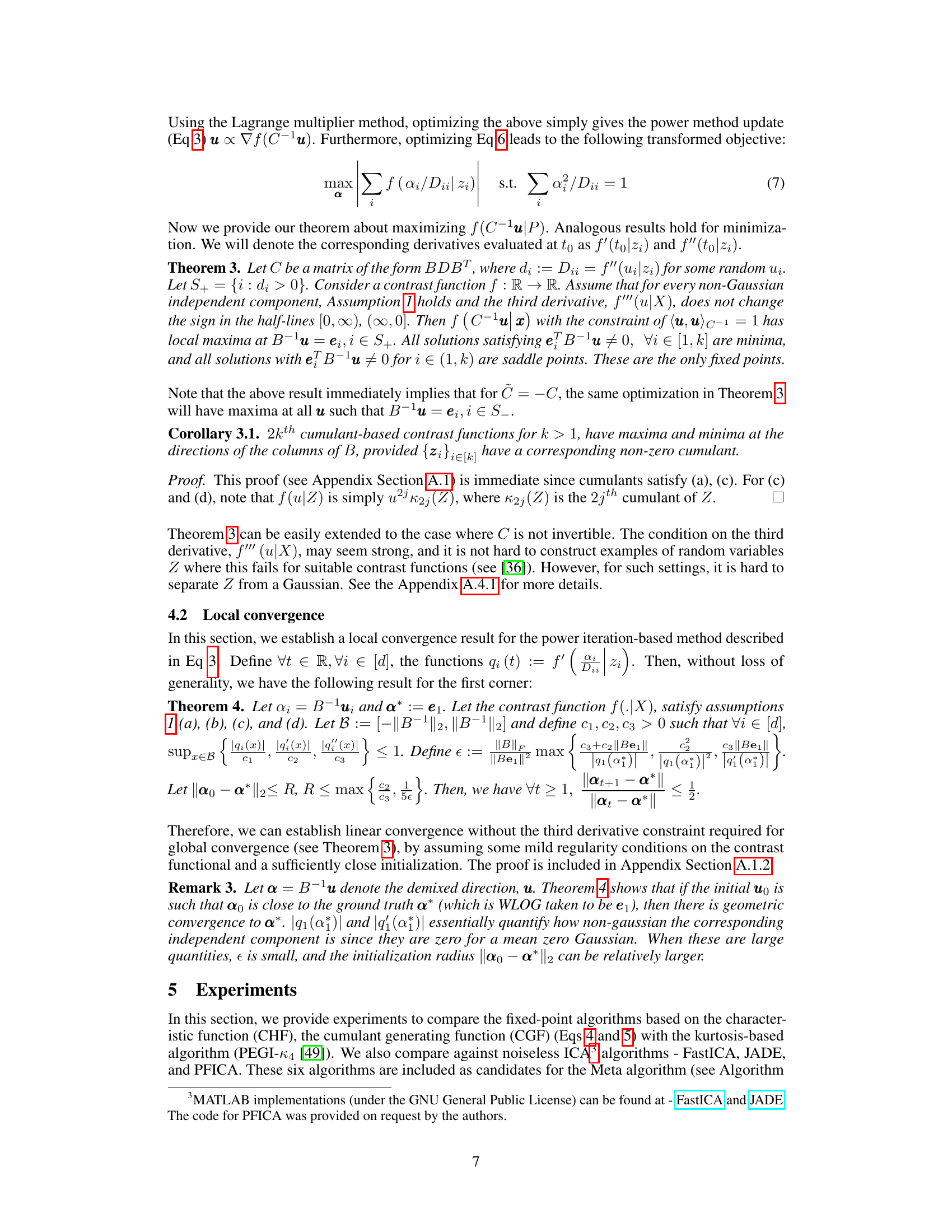
A convergence analysis in a machine learning context, particularly within the realm of Independent Component Analysis (ICA), is crucial for establishing the reliability and efficiency of proposed algorithms. A thorough analysis would delve into both global and local convergence properties. Global convergence examines whether the algorithm will eventually find a solution regardless of the starting point, while local convergence investigates how quickly it approaches a solution once it’s in a sufficiently close proximity. Theoretical guarantees regarding convergence rates and conditions for convergence are highly valuable, providing a strong foundation for algorithm’s trustworthiness. The analysis should address challenges posed by noisy data, which often complicates convergence. Furthermore, investigating the impact of hyperparameters and data characteristics on convergence behavior is essential to guide practical implementation. Simulations and empirical studies serve to complement theoretical analyses, providing practical insights and validating the findings. Finally, identifiability issues intrinsic to ICA, concerning the uniqueness of the recovered sources, should be considered within the convergence framework. A comprehensive analysis would blend rigorous theoretical analysis with well-designed experiments to provide a holistic understanding of the algorithm’s behavior and limitations.
Empirical Results#
An ‘Empirical Results’ section in a research paper would present the findings from experiments conducted to validate the paper’s claims. A strong section would begin by clearly stating the experimental setup, including datasets used, evaluation metrics employed, and any relevant hyperparameters. The presentation of results should be concise and well-organized, often using tables and figures to effectively showcase key findings. Visualizations, such as graphs and charts, are crucial for effectively communicating trends and comparisons between different methods or conditions. The discussion should focus on interpreting the results, highlighting statistically significant differences and comparing performance against relevant baselines. It’s vital to acknowledge any limitations or unexpected results. The section must directly relate to the hypotheses or claims presented in the introduction, providing strong evidence to support or refute them. A nuanced discussion that acknowledges both strengths and weaknesses of the findings would elevate the credibility of the research and contribute to a more complete understanding of the studied phenomena.
More visual insights#
More on figures

🔼 Figure 2 displays the results of experiments conducted to illustrate the variance reduction achieved using the Meta algorithm. The top panel (a) shows a histogram of the Amari error scores obtained from 40 independent runs of the CHF algorithm, each using a single random initialization. The bottom panel (b) shows a histogram of the Amari error scores, where, for each experiment, the best result out of 30 random initializations was selected using the independence score. The means and standard deviations of the histograms are (0.51, 0.51) and (0.39, 0.34) respectively, indicating a notable variance reduction and improved performance by using the independence score to choose the best results from multiple initializations.
read the caption
Figure 2: Histograms of Amari error with n = 104 and noise power p = 0.2

🔼 Figure 2(a) shows the variation of performance with noise power and Figure 2(b) shows the variation of performance with sample size. The histograms in Figure 2(c) compares the distribution of Amari error when using a single random initialization versus using multiple random initializations and choosing the best one using the independence score. The top panel shows that the Amari error for the CHF algorithm with one run has a mean of 0.51 and a standard deviation of 0.51. The bottom panel shows that the Amari error is reduced to a mean of 0.39 and standard deviation of 0.34 when using the independence score to select the best out of 30 runs.
read the caption
Figure 2: Histograms of Amari error with n = 104 and noise power p = 0.2

🔼 This figure demonstrates image demixing using ICA. Four source images are mixed using a 4x4 mixing matrix with added Wishart noise. The CHF-based method successfully recovers the original images, while the Kurtosis-based method fails to fully recover one source image. The Meta algorithm, which uses the independence score, selects CHF as the best-performing method.
read the caption
Figure 3: We demix images using ICA by flattening and linearly mixing them with a 4 × 4 matrix B (i.i.d entries ~ N(0, 1)) and Wishart noise (p = 0.001). The CHF-based method (c) recovers the original sources well, upto sign. The Kurtosis-based method (d) fails to recover the second source. This is consistent with its higher independence score. The Meta algorithm selects CHF from candidates CHF, CGF, Kurtosis, FastICA, and JADE. Appendix Section A.2 provides results for other contrast functions and their independence scores.

🔼 This figure demonstrates image demixing using ICA. Four images are mixed together, then separated using different ICA methods (CHF, Kurtosis, and two others). The CHF-based method produces the best results, accurately recovering the original images. This success is linked to its lower independence score, which is used by the Meta-algorithm to choose between the different ICA approaches.
read the caption
Figure 3: We demix images using ICA by flattening and linearly mixing them with a 4 × 4 matrix B (i.i.d entries ~ N(0, 1)) and Wishart noise (p = 0.001). The CHF-based method (c) recovers the original sources well, upto sign. The Kurtosis-based method (d) fails to recover the second source. This is consistent with its higher independence score. The Meta algorithm selects CHF from candidates CHF, CGF, Kurtosis, FastICA, and JADE.

🔼 This figure shows the results of image demixing using different ICA methods. Four source images are mixed together using a random 4x4 mixing matrix and added Wishart noise. Then, four different ICA methods (CHF, Kurtosis, CGF, and the Meta algorithm) are applied to recover the source images from the mixture. The CHF-based method performs the best, accurately recovering the source images. The Kurtosis-based method fails to recover one of the sources, highlighting the impact of choosing the right method for a given dataset. The Meta algorithm automatically selects the best performing method (CHF in this case).
read the caption
Figure 3: We demix images using ICA by flattening and linearly mixing them with a 4 × 4 matrix B (i.i.d entries ~ N(0, 1)) and Wishart noise (p = 0.001). The CHF-based method (c) recovers the original sources well, upto sign. The Kurtosis-based method (d) fails to recover the second source. This is consistent with its higher independence score. The Meta algorithm selects CHF from candidates CHF, CGF, Kurtosis, FastICA, and JADE.

🔼 This figure shows the results of image demixing using different ICA methods. Four images are mixed together, then demixed using four different methods: CHF-based, Kurtosis-based, CGF-based, and the Meta algorithm. The CHF-based method produces the best results, recovering the original images well, while the Kurtosis-based method fails to recover one of the sources, illustrating the effectiveness of the CHF method and the Meta algorithm in choosing the appropriate ICA method for a given dataset.
read the caption
Figure 3: We demix images using ICA by flattening and linearly mixing them with a 4 × 4 matrix B (i.i.d entries ~ N(0, 1)) and Wishart noise (p = 0.001). The CHF-based method (c) recovers the original sources well, upto sign. The Kurtosis-based method (d) fails to recover the second source. This is consistent with its higher independence score. The Meta algorithm selects CHF from candidates CHF, CGF, Kurtosis, FastICA, and JADE.

🔼 This figure shows the results of applying different ICA methods to a mixture of images. The top row shows the original source images, while the second row shows the mixed images. The bottom rows demonstrate the results of applying various ICA methods, including CHF, Kurtosis, and the Meta algorithm. The CHF-based method successfully separates the images, while the Kurtosis-based method fails to fully separate one of the sources. This difference is consistent with the independence scores computed for each method. The Meta algorithm successfully selects the best performing method in this case.
read the caption
Figure 3: We demix images using ICA by flattening and linearly mixing them with a 4 × 4 matrix B (i.i.d entries ~ N(0, 1)) and Wishart noise (p = 0.001). The CHF-based method (c) recovers the original sources well, upto sign. The Kurtosis-based method (d) fails to recover the second source. This is consistent with its higher independence score. The Meta algorithm selects CHF from candidates CHF, CGF, Kurtosis, FastICA, and JADE. Appendix Section A.2 provides results for other contrast functions and their independence scores.

🔼 This figure shows an example of image demixing using ICA. Four source images are mixed together using a random mixing matrix and added noise. The CHF-based ICA method successfully separates the mixed images into their original components, while the Kurtosis-based method fails to recover one of the sources. The Meta algorithm, which adaptively selects the best ICA algorithm based on an independence score, correctly chooses the CHF-based method in this case.
read the caption
Figure 3: We demix images using ICA by flattening and linearly mixing them with a 4 × 4 matrix B (i.i.d entries ~ N(0, 1)) and Wishart noise (p = 0.001). The CHF-based method (c) recovers the original sources well, upto sign. The Kurtosis-based method (d) fails to recover the second source. This is consistent with its higher independence score. The Meta algorithm selects CHF from candidates CHF, CGF, Kurtosis, FastICA, and JADE.

🔼 This figure shows the results of image demixing using ICA with different contrast functions. The images are first mixed using a 4x4 mixing matrix and added Wishart noise. Then, different ICA methods (CHF, Kurtosis, CGF, FastICA, JADE) are used to recover the original images. The CHF-based method shows the best performance in recovering the original sources.
read the caption
Figure 3: We demix images using ICA by flattening and linearly mixing them with a 4 × 4 matrix B (i.i.d entries ~ N(0, 1)) and Wishart noise (p = 0.001). The CHF-based method (c) recovers the original sources well, upto sign. The Kurtosis-based method (d) fails to recover the second source. This is consistent with its higher independence score. The Meta algorithm selects CHF from candidates CHF, CGF, Kurtosis, FastICA, and JADE.

🔼 This figure shows the results of applying different ICA methods to a set of mixed images. The images were mixed using a random 4x4 matrix and added Wishart noise. The CHF (Characteristic Function)-based method successfully separates the source images, while the Kurtosis-based method fails. The Meta algorithm, which uses an independence score to select the best method, correctly chooses the CHF method in this case. This demonstrates the effectiveness of the proposed independence score and Meta algorithm.
read the caption
Figure 3: We demix images using ICA by flattening and linearly mixing them with a 4 × 4 matrix B (i.i.d entries ~ N(0, 1)) and Wishart noise (p = 0.001). The CHF-based method (c) recovers the original sources well, upto sign. The Kurtosis-based method (d) fails to recover the second source. This is consistent with its higher independence score. The Meta algorithm selects CHF from candidates CHF, CGF, Kurtosis, FastICA, and JADE.

🔼 This figure shows the results of image denoising experiments using different ICA-based methods. The original noisy MNIST images are shown in (a). The denoised images obtained using CHF, Kurtosis, CGF, FastICA, and JADE methods are displayed in (b) through (f) respectively. Each denoising result is accompanied by its independence score, indicating the quality of denoising. The CHF-based method demonstrates superior performance compared to other methods, having a considerably lower independence score, signifying better separation of noise from the image data.
read the caption
Figure A.2: Image Denoising using ICA
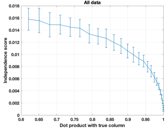
🔼 This figure shows the relationship between the independence score and the dot product of a vector with a true column of the mixing matrix. The independence score is a measure of how independent the estimated components are, and a lower score is desired. The dot product measures how aligned the vector is with a true column; a higher dot product indicates better alignment. The figure demonstrates that as the dot product increases (i.e., the estimated vector is more aligned with the true vector), the independence score decreases, indicating higher independence of the estimated components. Error bars are shown for each data point. This illustrates the relationship between the quality of ICA estimations and the independence score in the proposed algorithm.
read the caption
Figure A.3: Mean independence score with errorbars from 50 random runs
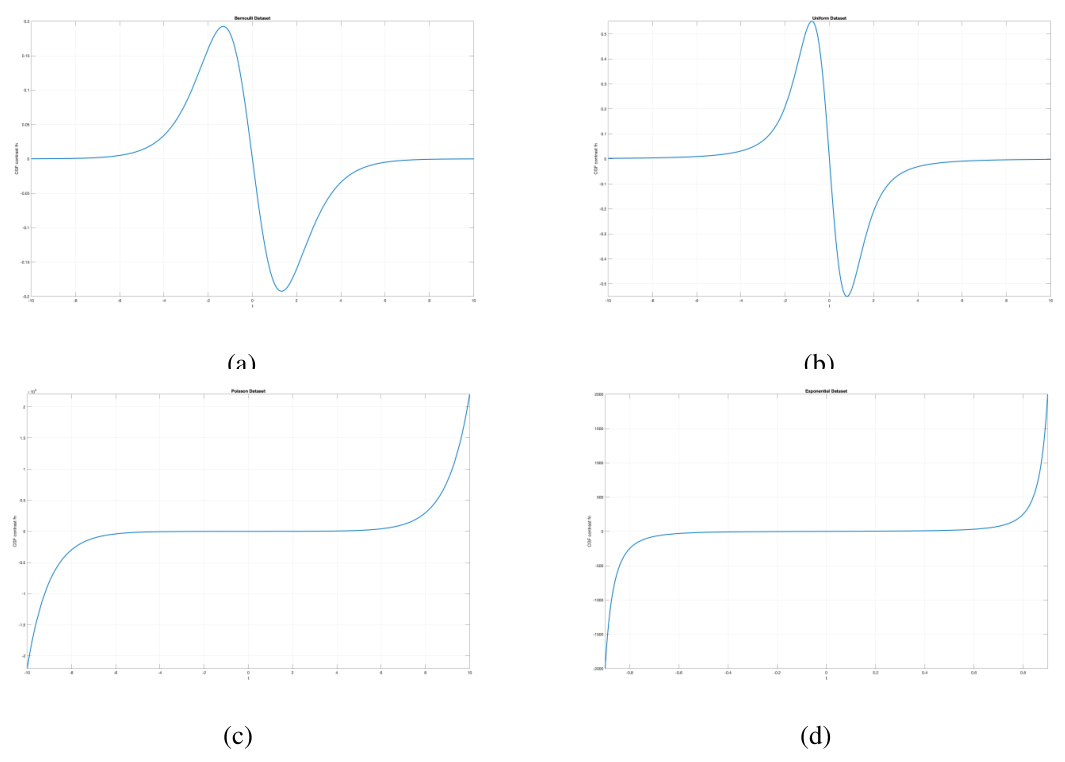
🔼 The figure shows the plots of the third derivative of the CGF-based contrast function for four different distributions: Bernoulli, Uniform, Poisson, and Exponential. The plots demonstrate that the sign of the third derivative remains consistent within each half-line (positive or negative values) for each distribution, fulfilling a key condition of Theorem 3.
read the caption
Figure A.4: Plots of the third derivative of the CGF-based contrast function for different datasets - Bernoulli(p = 0.5) A.4a, Uniform(U(−√3, √3)) A.4b, Poisson(λ = 1) A.4c and Exponential(λ = 1) A.4d. Note that the sign stays the same in each half-line

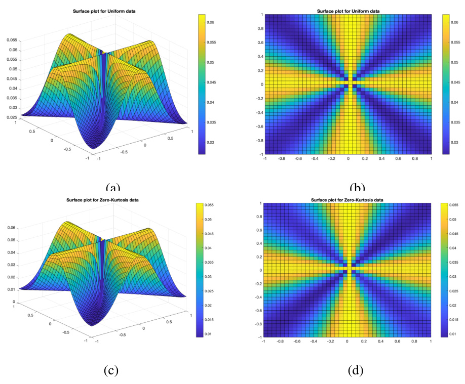
🔼 This figure shows surface plots of the loss landscape for the CHF-based contrast function. It visualizes the contrast function’s values across a range of u (the vector in the pseudo-Euclidean space used for optimization). The plots are for both zero-kurtosis and uniform data, illustrating the behavior of the function in different scenarios. Global maxima are observed when u aligns with the columns of the mixing matrix B, indicating the function’s effectiveness in identifying the underlying independent components.
read the caption
Figure A.6: Surface plots for zero-kurtosis (A.6c and A.6d) and Uniform (A.6a, A.6b) data with n = 10000 points, noise-power p = 0.1 and number of source signals, k = 2.
🔼 This figure presents the results of experiments evaluating the performance of the proposed independence score and Meta algorithm, illustrating the impact of varying noise levels and sample sizes on the accuracy of Independent Component Analysis (ICA). It also demonstrates the variance reduction achieved by selecting the best-performing run from multiple random initializations using the independence score.
read the caption
Figure 2: Histograms of Amari error with varying noise powers (for n = 105) and varying sample sizes (for p = 0.2) on x axis for figures 2a and 2b respectively. For figure 2c, the top panel contains a histogram of 40 runs with one random initialization. The bottom panel contains a histogram of 40 runs, each of which is the best independence score out of 30 random initializations.
More on tables

🔼 This table shows the median Amari error for different algorithms across various Bernoulli distributions. The scaled kurtosis is also provided. The Meta algorithm, which adaptively selects the best algorithm based on a new independence score, is shown to perform as well or better than the best individual algorithm in most cases. Note that FastICA failed to converge when the kurtosis was zero.
read the caption
Table 1: Median Amari error with varying p in Bernoulli(p) data. The scaled kurtosis is given as κ4 := (1 – 6p(1 − p))/(p(1 − p)). Observe that the Meta algorithm (shaded in red) performs at par or better than the best candidate algorithms. FastICA did not converge for zero-kurtosis data.

🔼 This table shows the median Amari error for different algorithms across various values of p in a Bernoulli(p) distribution. The scaled kurtosis is also provided, highlighting the performance of each algorithm under varying levels of kurtosis. The Meta algorithm, which uses a score to select the best-performing algorithm, consistently achieves performance at least as good as the best individual algorithm. Notably, FastICA failed to converge when the kurtosis was zero.
read the caption
Table 1: Median Amari error with varying p in Bernoulli(p) data. The scaled kurtosis is given as K4 := (1 – 6p(1 − p))/(p(1 − p)). Observe that the Meta algorithm (shaded in red) performs at par or better than the best candidate algorithms. FastICA did not converge for zero-kurtosis data.
Full paper#

