TL;DR#
Physics-Informed Neural Networks (PINNs) demonstrate great promise for solving partial differential equations, but often suffer from training instability due to gradient issues. Specifically, gradients from different loss functions (boundary and PDE residual losses) can exhibit significant magnitude imbalances and negative inner products, leading to unreliable solutions. This is a critical challenge hindering wider adoption of PINNs.
To tackle this issue, this paper introduces a new optimization framework called Dual Cone Gradient Descent (DCGD). DCGD cleverly adjusts the gradient update direction to ensure that both boundary and PDE residual losses decrease simultaneously. Theoretical convergence properties are analyzed, demonstrating its effectiveness in non-convex settings. Extensive experiments across various benchmark equations showcase DCGD’s superior performance and stability compared to existing methods, especially for complex PDEs and failure modes of PINNs.
Key Takeaways#
Why does it matter?#
This paper is crucial for researchers working with Physics-Informed Neural Networks (PINNs). It addresses the common problem of PINN training instability caused by gradient imbalance, offering a novel optimization framework (DCGD) that significantly improves accuracy and reliability. This work is highly relevant to the current trends in scientific machine learning and opens new avenues for improving multi-objective optimization in deep learning.
Visual Insights#
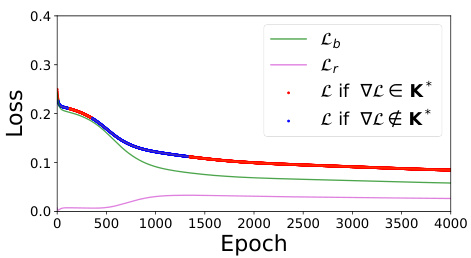
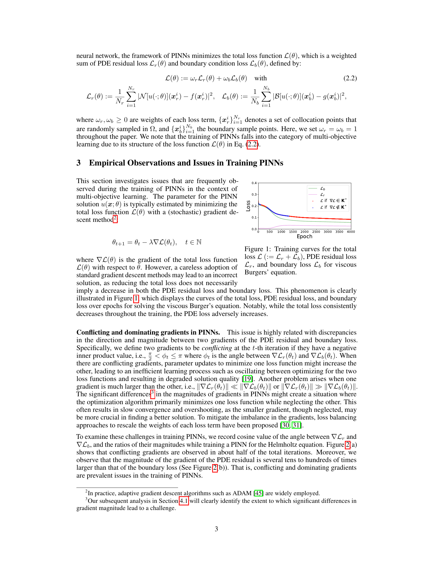
🔼 This figure shows the training curves of total loss, PDE residual loss, and boundary loss for solving viscous Burgers’ equation. It illustrates how the total loss consistently decreases, while PDE loss increases at a certain point during training. This highlights the issue of conflicting gradients and imbalance between losses in training PINNs.
read the caption
Figure 1: Training curves for the total loss L (:= Lr + Lb), PDE residual loss Lr, and boundary loss Lb for viscous Burgers' equation.

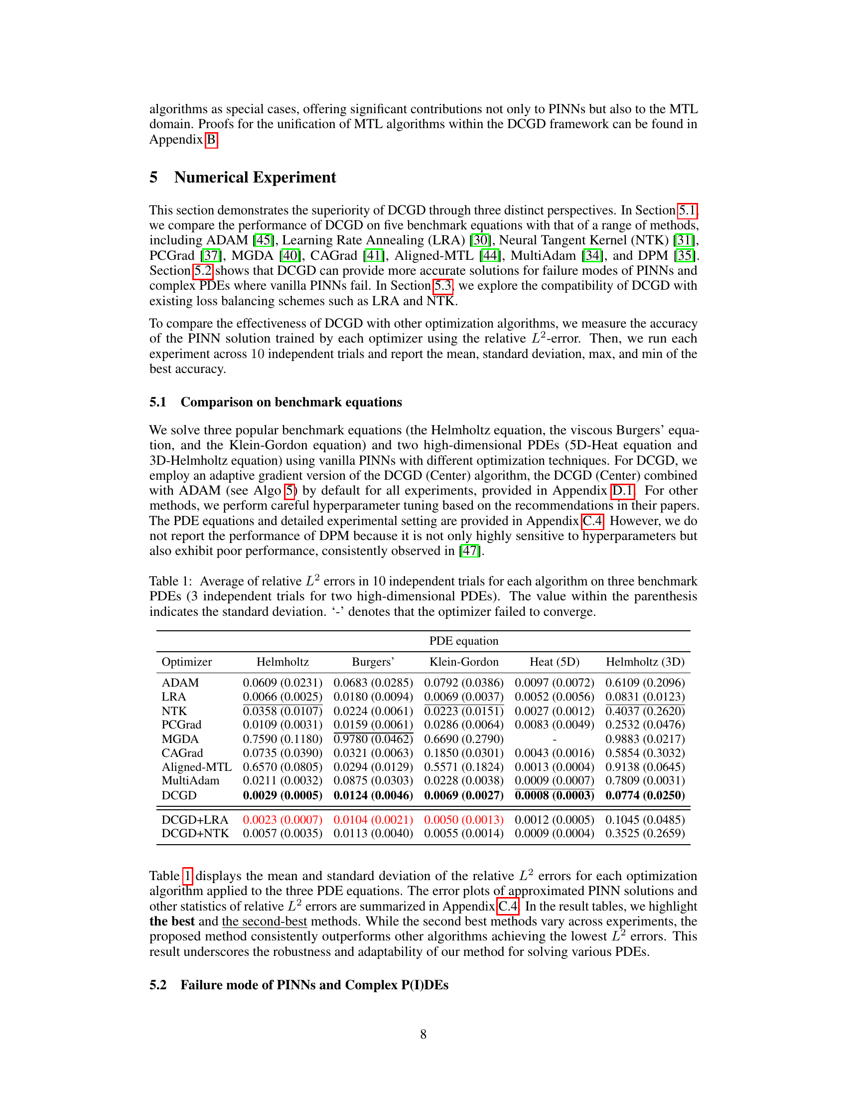
🔼 This table presents the mean and standard deviation of the relative L2 error for several optimization algorithms used to solve various partial differential equations (PDEs). The PDEs include the Helmholtz equation, the viscous Burgers’ equation, the Klein-Gordon equation, the 5D-Heat equation, and the 3D-Helmholtz equation. The algorithms compared include ADAM, LRA, NTK, PCGrad, MGDA, CAGrad, Aligned-MTL, MultiAdam, and DCGD (with and without LRA and NTK). Lower relative L2 error values indicate better performance of the optimization algorithm.
read the caption
Table 1: Average of relative L2 errors in 10 independent trials for each algorithm on three benchmark PDEs (3 independent trials for two high-dimensional PDEs). The value within the parenthesis indicates the standard deviation. '-' denotes that the optimizer failed to converge.
In-depth insights#
PINN Pathologies#
Physics-Informed Neural Networks (PINNs) demonstrate potential in solving Partial Differential Equations (PDEs); however, pathological behaviors hinder their reliability. These pathologies manifest as the model failing to converge to a reasonable solution or converging to a trivial solution that doesn’t satisfy the governing PDE. Gradient imbalance, where gradients from the PDE residual loss and boundary conditions have significantly different magnitudes, is a major contributor. This imbalance can lead to conflicting updates during training, causing oscillations or slow convergence. The negative inner product between the gradients further exacerbates this issue. Dominating gradients also pose a significant challenge; one loss term may dominate the optimization process to the detriment of the other, resulting in an incomplete or incorrect solution. Addressing these pathologies requires a deeper understanding of their root causes and innovative strategies, such as methods that adjust gradient directions to improve the balance between loss terms. Understanding and resolving these pathologies is crucial to enhance the robustness and reliability of PINNs for solving complex scientific and engineering problems.
Dual Cone Descent#
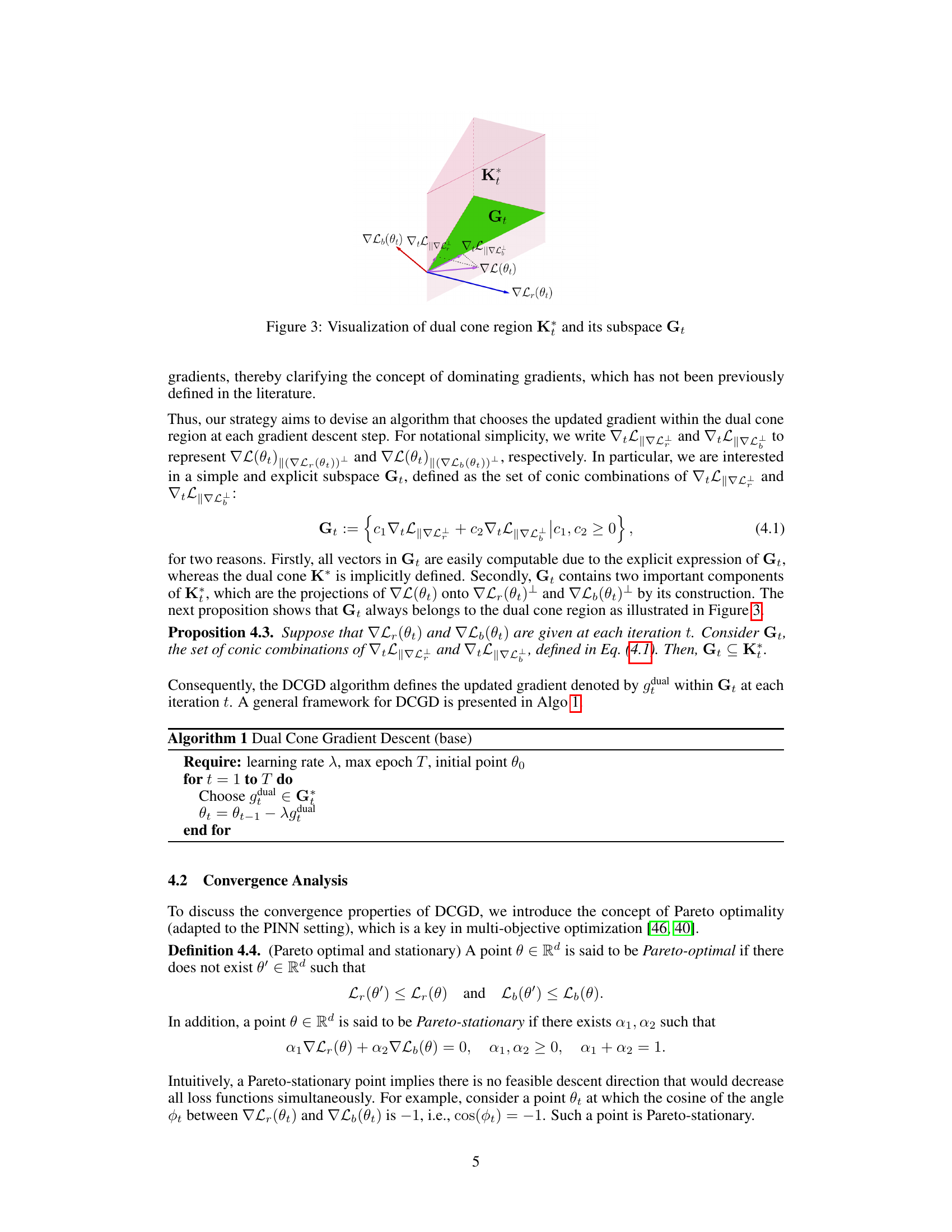
The concept of “Dual Cone Descent” in the context of training Physics-Informed Neural Networks (PINNs) offers a novel approach to address the challenges of gradient imbalance and conflicting gradients that often hinder PINN performance. The core idea is to constrain the gradient updates within a dual cone region, where the inner products of the updated gradient with both PDE residual loss and boundary loss gradients remain non-negative. This ensures that updates simultaneously reduce both loss components, preventing the detrimental oscillations and imbalances often observed in standard PINN training. The dual cone itself is defined by the gradients of the two loss terms, providing a geometric interpretation to the optimization process. This geometric perspective enables a deeper understanding of the training dynamics and offers a principled way to resolve the gradient conflicts commonly encountered in multi-objective optimization problems inherent in PINN training. Furthermore, the theoretical analysis of convergence properties for algorithms built upon this dual cone framework adds rigorous support, establishing its potential for robust and reliable training of PINNs. The proposed framework can be extended to various existing PINN methodologies, further enhancing its flexibility and applicability to a wide range of complex PDEs.
Convergence Analysis#
A rigorous convergence analysis is crucial for establishing the reliability and effectiveness of any optimization algorithm. In the context of the research paper, a convergence analysis of the proposed Dual Cone Gradient Descent (DCGD) algorithm is vital for understanding its theoretical guarantees and its practical performance. The analysis should ideally cover scenarios where the objective function is non-convex, reflecting the challenging nature of training physics-informed neural networks (PINNs). A key aspect of the convergence analysis would be to define appropriate convergence criteria that align with the multi-objective nature of the PINN training problem. The analysis needs to address the convergence to a Pareto-stationary point or to other stationary points, as the standard notion of convergence to a single optimal solution may not be directly applicable. The theoretical analysis should be complemented with empirical validation, demonstrating the algorithm’s convergence behavior across various benchmarks and failure modes of PINNs. Demonstrating both convergence speed and stability is key, showcasing that the algorithm not only finds a solution but also does so efficiently and reliably, even in complex scenarios. The convergence analysis should provide valuable insights into the algorithm’s behavior, improving the understanding of its strengths and limitations.
Empirical Validation#
An Empirical Validation section in a research paper would rigorously test the proposed methods. It would likely involve experiments on diverse benchmark datasets, comparing performance against state-of-the-art techniques using relevant metrics. A strong validation would show consistent improvements across multiple datasets and demonstrate robustness to variations in parameters or data characteristics. Detailed analyses of the results, including statistical significance tests and error bars, would be critical to support the paper’s claims. Visualizations like graphs or tables presenting results clearly and concisely would be essential for reader understanding. The section should also address any limitations of the validation methodology, for example, if some datasets are better suited to the method than others, or potential biases. A robust empirical validation builds strong confidence in the applicability and effectiveness of the presented methods, contributing significantly to the paper’s overall credibility and impact.
Future of PINNs#
The future of Physics-Informed Neural Networks (PINNs) is bright, but also faces challenges. Improved optimization techniques, such as the Dual Cone Gradient Descent (DCGD) method, are crucial for addressing issues like gradient imbalance and instability during training. Addressing limitations in handling complex PDEs and failure modes remains a priority, requiring further research into adaptive loss balancing and innovative gradient manipulation strategies. Expanding the applications of PINNs to broader scientific domains and incorporating them with other advanced machine learning methods, such as transformers, holds significant promise. Enhanced computational efficiency is also essential, especially when tackling high-dimensional PDEs, possibly through advanced architectures and specialized hardware acceleration. Finally, developing robust theoretical frameworks that explain the behavior of PINNs and guide their development is critical for achieving broader adoption and trust in their capabilities.
More visual insights#
More on figures

🔼 This figure shows the distribution of the cosine of the angle (φ) between the gradients of the PDE residual loss (∇Lr) and the boundary loss (∇Lb) during the training of PINNs, as well as the distribution of the ratio (R) of their magnitudes. The left histogram illustrates the prevalence of conflicting gradients (cos(φ) < 0). The right histogram shows that the magnitude of the PDE residual gradient frequently dominates the boundary loss gradient, indicating a significant imbalance that can hinder effective training.
read the caption
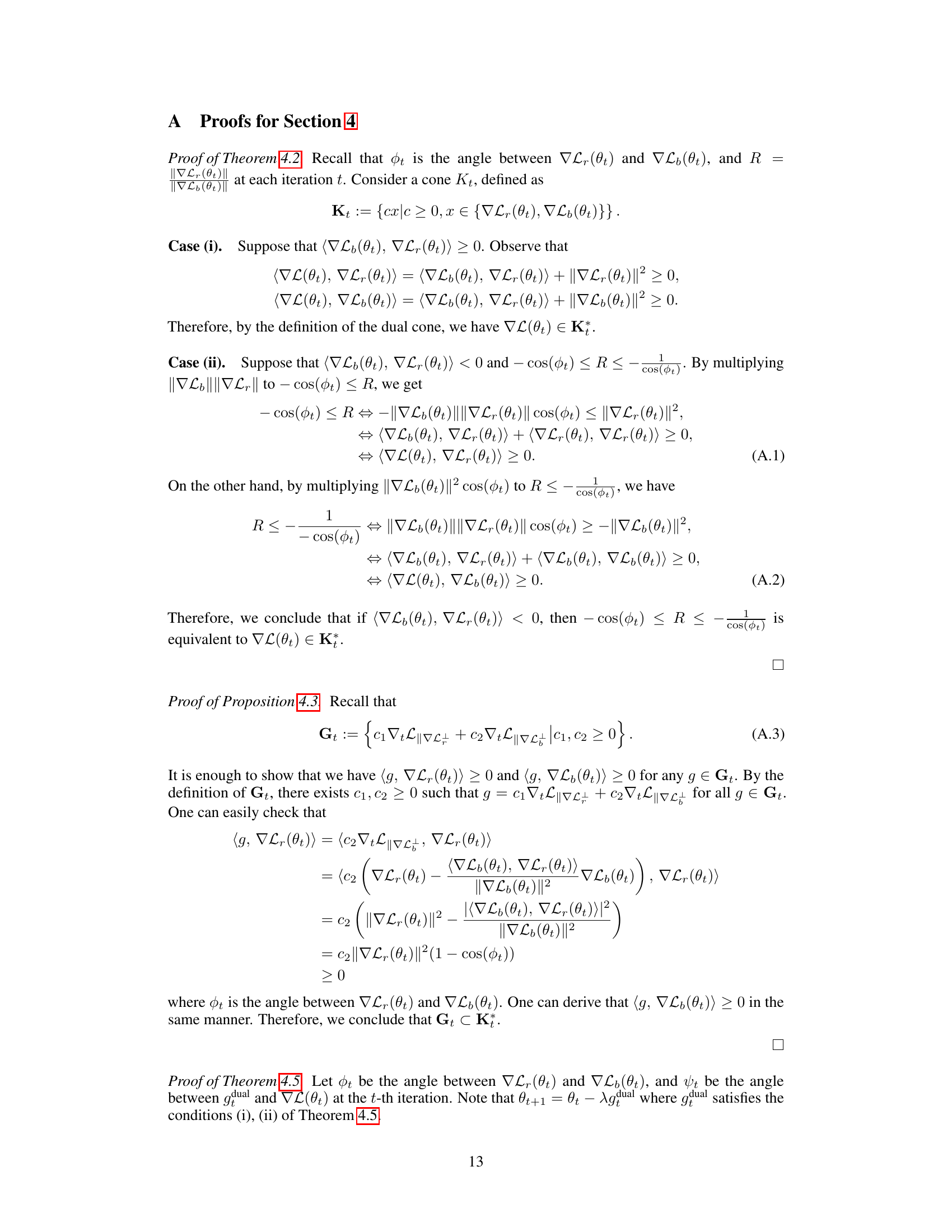
Figure 2: Conflicting and dominating gradients in PINNs. Here, φ is defined as the angle between ∇Lr and ∇Lb, R = ||∇Lr||/||∇Lb|| is the magnitude ratio between gradients.
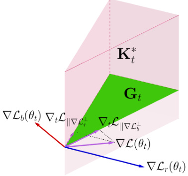
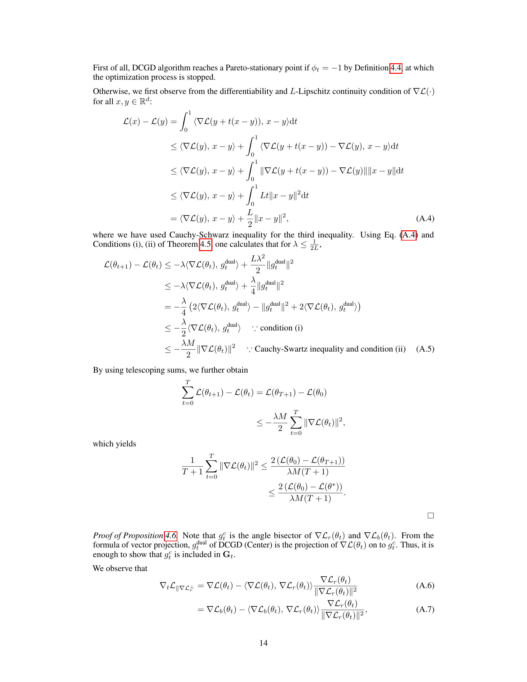
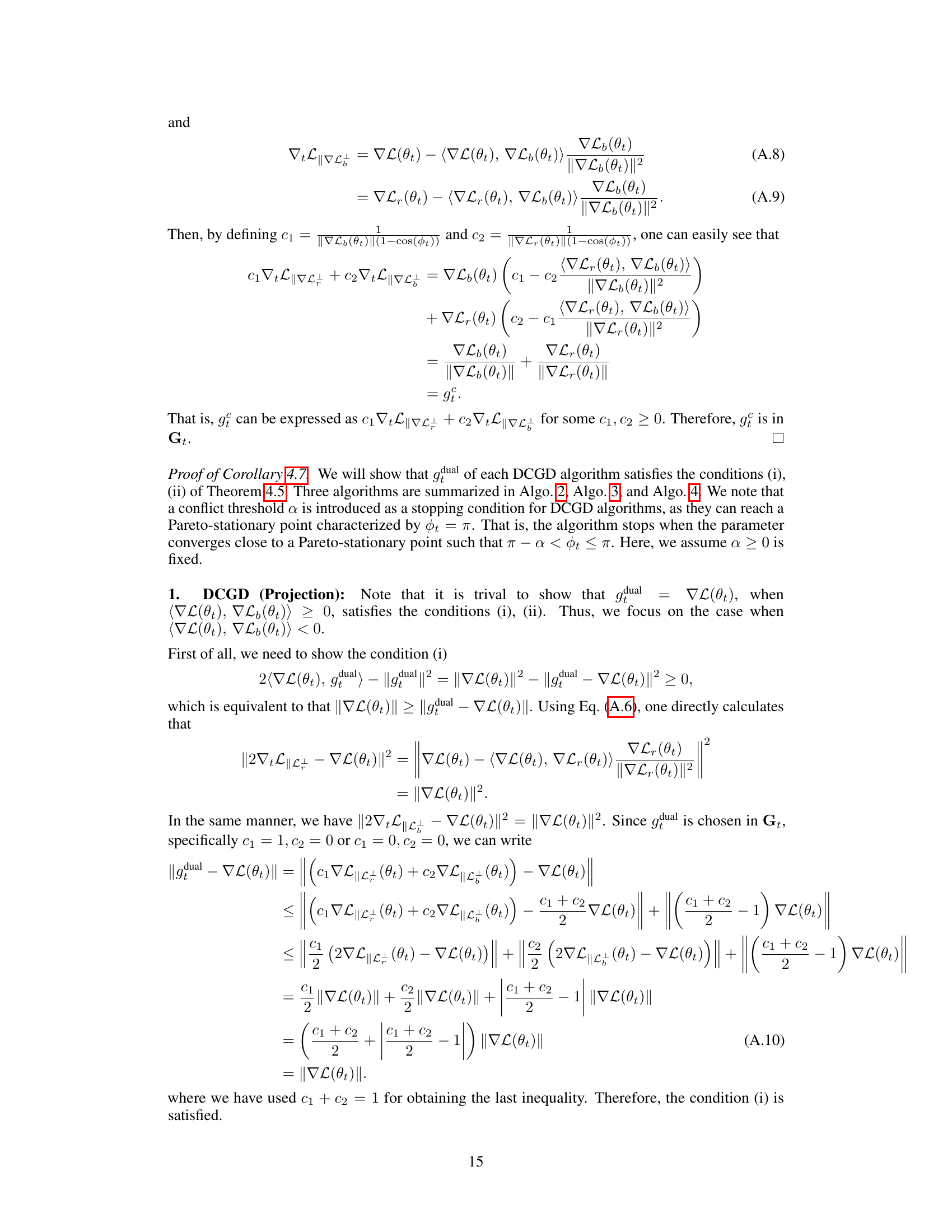
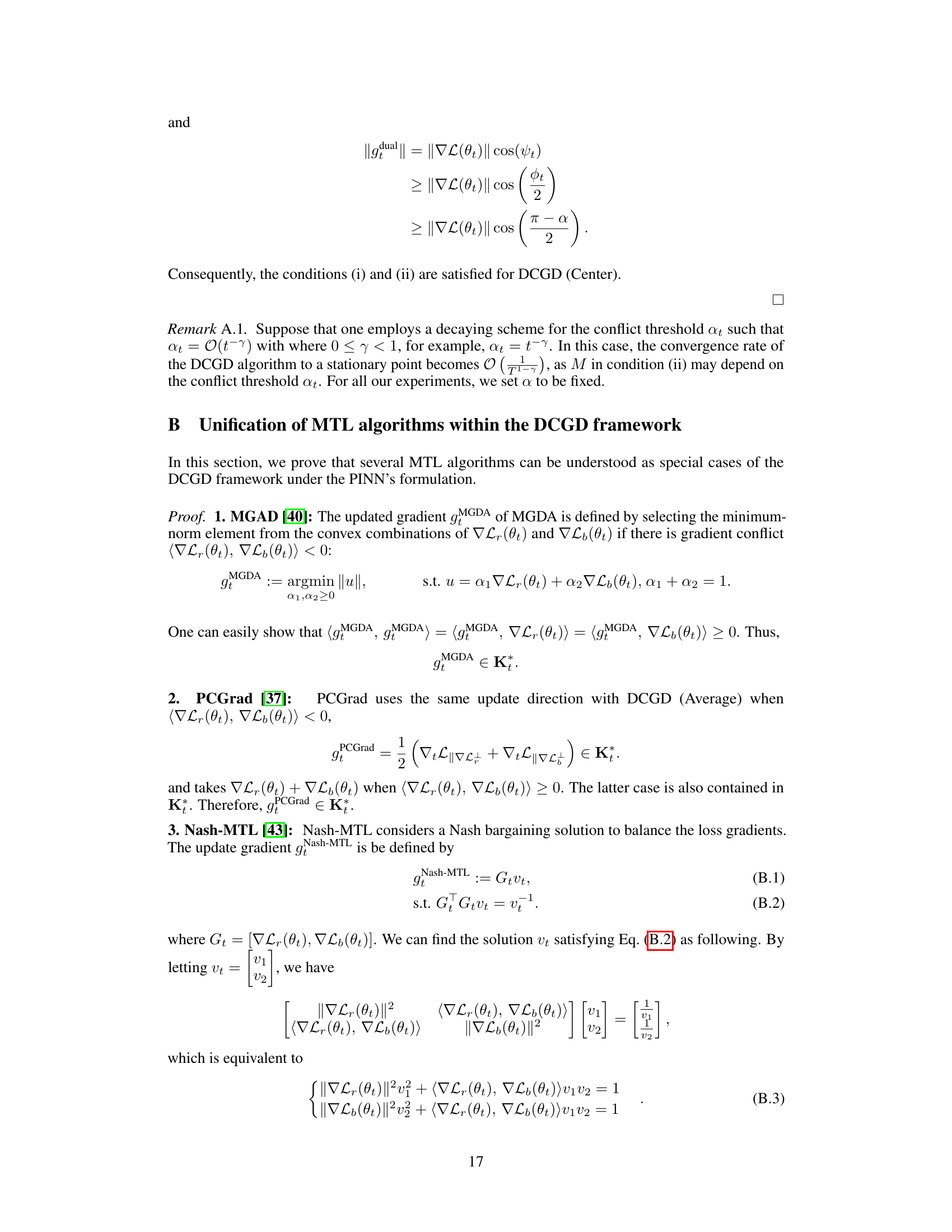
🔼 This figure visualizes the dual cone region Kt and its subspace Gt. The dual cone Kt is the set of vectors that have non-negative inner products with all vectors in the cone Kt, which is generated by the gradients of the PDE residual loss and the boundary loss. The subspace Gt is a subset of K*t, defined as the set of conic combinations of the projections of the total gradient onto the orthogonal complements of the PDE residual loss gradient and boundary loss gradient. The figure illustrates how the updated gradient (gdual) in the DCGD algorithm is chosen to ensure it lies within Gt, guaranteeing simultaneous decrease in both PDE residual loss and boundary loss.
read the caption
Figure 3: Visualization of dual cone region K*t and its subspace Gt

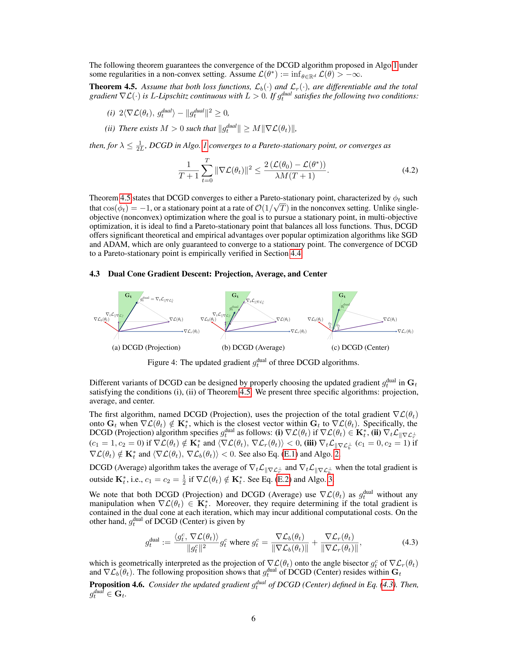
🔼 This figure visualizes how the updated gradient (gdual) is determined in three different variants of the Dual Cone Gradient Descent (DCGD) algorithm: Projection, Average, and Center. Each subfigure shows a different strategy for selecting gdual within the dual cone region (Gt) based on the gradients of the PDE residual loss and boundary loss. (a) DCGD (Projection) projects the total gradient onto the subspace Gt. (b) DCGD (Average) averages the projected gradients. (c) DCGD (Center) uses the angle bisector of the two gradients as the updated gradient. The visualization helps to understand the different approaches to ensure that the updated gradient remains within the dual cone, which guarantees that both losses can decrease simultaneously, avoiding the conflicting gradient issues during PINN training.
read the caption
Figure 4: The updated gradient gdual of three DCGD algorithms.

🔼 This figure shows the distribution of the cosine of the angle between the gradients of the PDE residual loss and the boundary loss (cos(φ)) and the ratio of their magnitudes (R) during the training process of PINNs for the Helmholtz equation. The histograms reveal that: (a) In approximately half of the iterations, the gradients are conflicting (cos(φ) < 0), indicating that reducing one loss increases the other. (b) The magnitude of the PDE residual gradient is often significantly larger than that of the boundary loss gradient (R » 1), implying that the optimization process is dominated by the PDE residual loss, potentially neglecting the boundary loss.
read the caption
Figure 2: Conflicting and dominating gradients in PINNs. Here, φ is defined as the angle between ∇Lr and ∇Lb, R = ||∇Lr||/||∇Lb|| is the magnitude ratio between gradients.

🔼 This figure shows histograms visualizing the distribution of the cosine of the angle (cos(φ)) between the gradients of the PDE residual loss (∇Lr) and the boundary loss (∇Lb) during the training process of Physics-Informed Neural Networks (PINNs). It also displays a histogram of the magnitude ratio (R) between the two gradients (||∇Lr||/||∇Lb||). The histograms illustrate that conflicting gradients (cos(φ) < 0) and gradients with a significant imbalance in magnitude (R being much greater than 1) are frequent occurrences during PINN training, suggesting a potential cause for training instability.
read the caption
Figure 2: Conflicting and dominating gradients in PINNs. Here, φ is defined as the angle between ∇Lr and ∇Lb, R = ||∇Lr||/||∇Lb|| is the magnitude ratio between gradients.

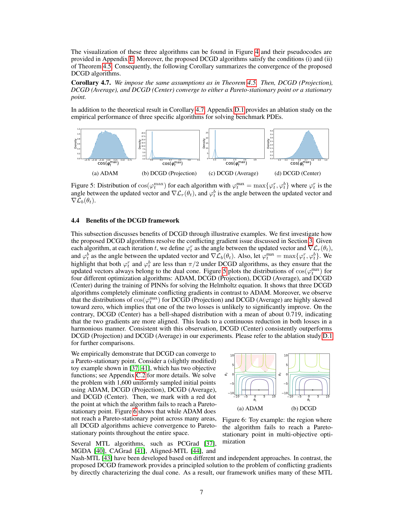
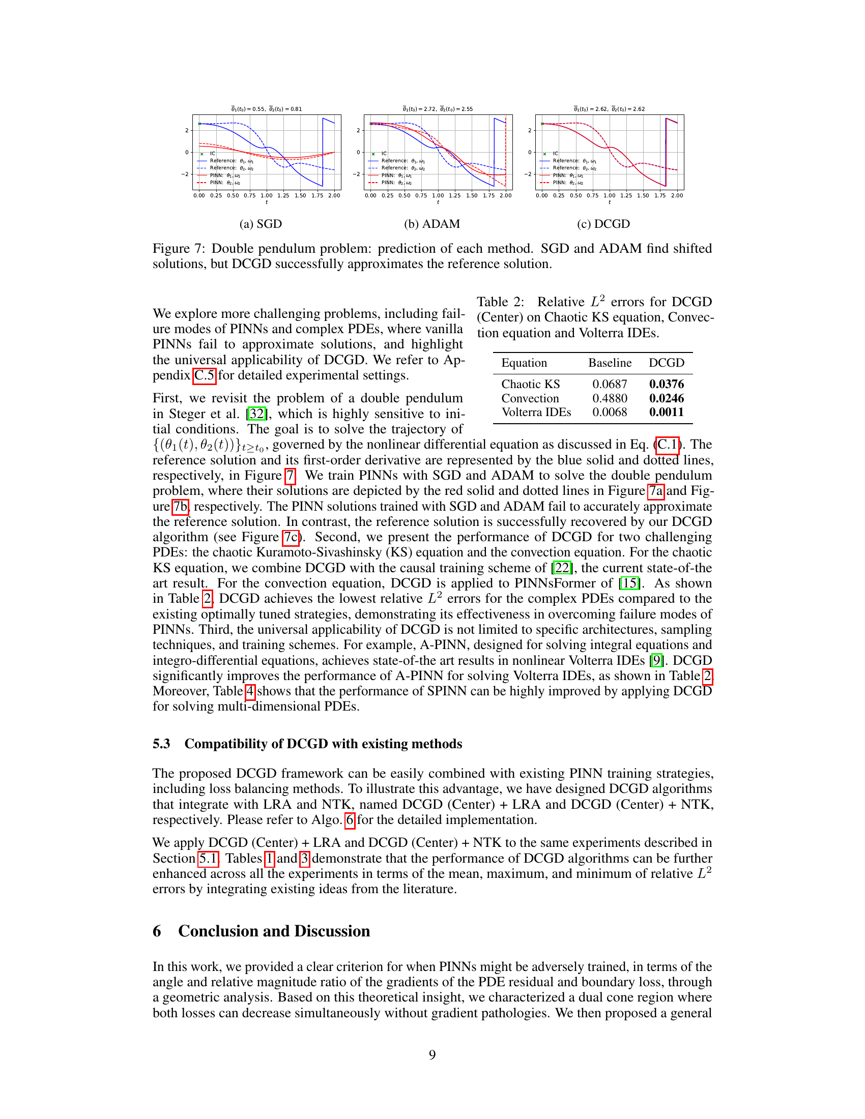
🔼 This figure compares the performance of three different optimization algorithms (SGD, ADAM, and DCGD) on the double pendulum problem. The plots show the predicted angles (θ1 and θ2) over time for each algorithm. The reference solution is shown in blue. SGD and ADAM fail to accurately predict the reference solution, exhibiting a significant shift in the predicted angles. In contrast, the DCGD algorithm closely matches the reference solution, indicating its superior ability to solve this challenging problem.
read the caption
Figure 7: Double pendulum problem: prediction of each method. SGD and ADAM find shifted solutions, but DCGD successfully approximates the reference solution.
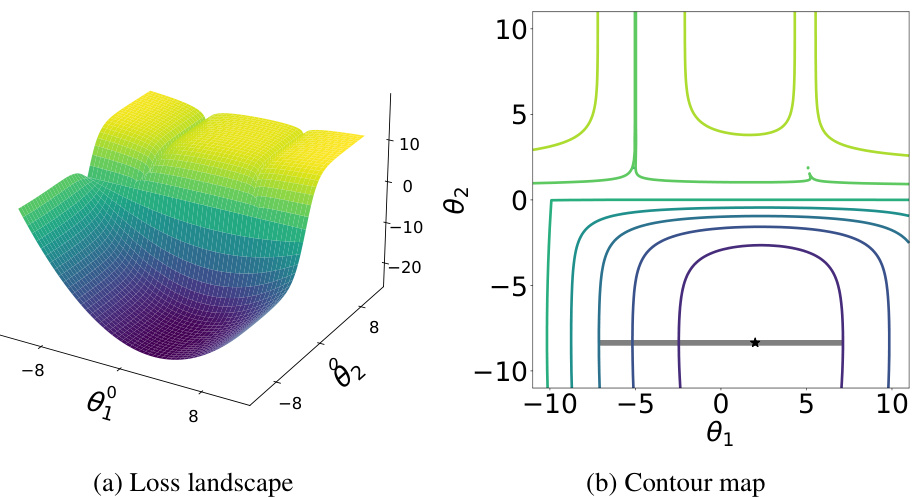
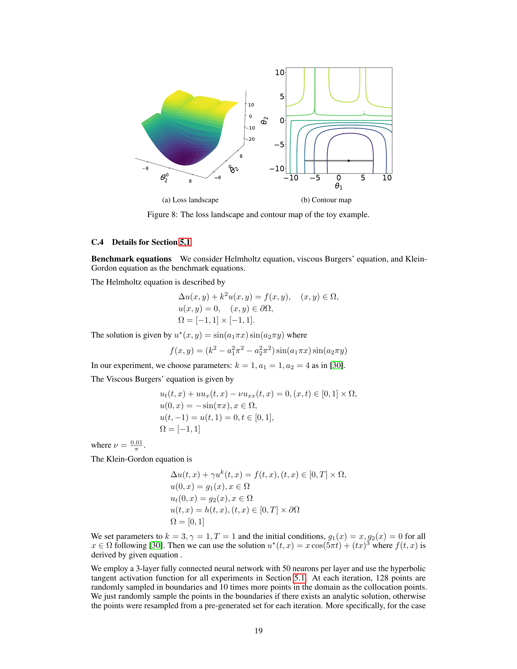
🔼 This figure visualizes the loss landscape and contour map of a toy example used in the paper to illustrate the challenges in training Physics-Informed Neural Networks (PINNs) and the benefits of the proposed Dual Cone Gradient Descent (DCGD) method. The loss landscape is a 3D surface showing how the total loss function varies with two parameters (θ₁ and θ₂). The contour map provides a 2D projection of the same data, showing the level curves of the loss function. The Pareto set (optimal solutions) is highlighted in gray in the contour map. This figure demonstrates how conflicting gradients can lead to failure in training PINNs and how DCGD can effectively resolve these issues.
read the caption
Figure 8: The loss landscape and contour map of the toy example.

🔼 This figure visualizes the results of solving the Helmholtz equation using Physics-Informed Neural Networks (PINNs). It compares the exact solution (a), the PINN’s prediction (b), and the absolute error between the two (c). The color map represents the magnitude of the solution, allowing for a visual comparison of the accuracy of the PINN’s approximation. This figure showcases the effectiveness of the proposed method in approximating solutions to partial differential equations.
read the caption
Figure 9: Helmholtz equation: approximated solution versus the reference solution.

🔼 This figure compares the exact solution, the PINN prediction, and the absolute error for the viscous Burgers’ equation. It visually demonstrates the accuracy of the Physics-Informed Neural Network (PINN) in approximating the solution of this benchmark partial differential equation. The plots show the solution across the spatial dimension (x) and the temporal dimension (t). The closeness of the prediction to the exact solution indicates the success of the PINN model in solving the given PDE.
read the caption
Figure 10: Burgers' equation: approximated solution versus the reference solution.

🔼 This figure visualizes the results of approximating the solution to the viscous Burgers’ equation using a physics-informed neural network (PINN). It includes three subplots: (a) shows the exact solution of the equation; (b) displays the solution predicted by the PINN; and (c) presents the absolute error between the exact and predicted solutions. The plots illustrate the PINN’s ability to approximate the solution, with subplot (c) quantifying the accuracy of the approximation.
read the caption
Figure 10: Burgers' equation: approximated solution versus the reference solution.

🔼 This figure shows a schematic of a simple double pendulum. It consists of two point masses (m1 and m2) connected by two massless rods of lengths l1 and l2. The angles θ1 and θ2 represent the angles that each rod makes with respect to the vertical. This system is used as an example in the paper to illustrate the challenges in training physics-informed neural networks.
read the caption
Figure 12: Simple double pendulum example

🔼 This figure shows the training curves of a physics-informed neural network (PINN) for solving the viscous Burgers’ equation. It plots the total loss, the PDE residual loss, and the boundary loss against the number of training epochs. The key observation is that while the total loss decreases consistently throughout training, the PDE loss increases at a certain point. This highlights one of the main challenges addressed in the paper: the imbalance and potential conflict between different loss terms during PINN training.
read the caption
Figure 1: Training curves for the total loss L (:= Lr + Lb), PDE residual loss Lr, and boundary loss Lb for viscous Burgers' equation.

🔼 This figure compares the exact solution, the solution predicted by the PINN model, and the absolute error between the two for the viscous Burgers’ equation. The plots show the solutions across the spatial dimension (x) and the temporal dimension (t). This visual comparison helps to assess the accuracy and effectiveness of the PINN model in solving the equation.
read the caption
Figure 10: Burgers' equation: approximated solution versus the reference solution.

🔼 This figure illustrates the issues of conflicting and dominating gradients in training Physics-Informed Neural Networks (PINNs). The left histogram shows the distribution of the cosine of the angle (φ) between the gradients of the PDE residual loss (∇Lr) and the boundary loss (∇Lb). A negative cosine indicates conflicting gradients, while values close to 1 indicate aligned gradients. The right histogram shows the distribution of the magnitude ratio (R) between the two gradients. A large R indicates that one gradient is significantly larger than the other, which can hinder effective training. The observation shows that conflicting gradients are prevalent in PINN training, and one gradient often dominates the other, leading to training instability and suboptimal solutions.
read the caption
Figure 2: Conflicting and dominating gradients in PINNs. Here, φ is defined as the angle between ∇Lr and ∇Lb, R = ||∇Lr||/||∇Lb|| is the magnitude ratio between gradients.

🔼 This figure compares the exact solution, the predicted solution by the SPINN model, and the absolute error between them for the 3D Helmholtz equation. The visualization is a 3D representation showing the solution across the x, y, and z dimensions. It provides a visual representation of the model’s accuracy in approximating the solution of this complex PDE.
read the caption
Figure 16: 3D-Helmholtz equation: approximated solution versus the reference solution.
More on tables
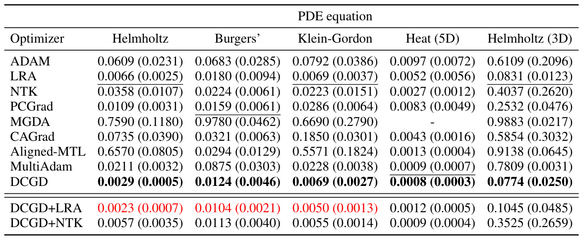
🔼 This table presents the mean and standard deviation of the relative L2 errors for various optimization algorithms applied to three benchmark PDEs (Helmholtz, Burgers’, Klein-Gordon) and two high-dimensional PDEs (5D Heat, 3D Helmholtz). The results are based on 10 independent trials (3 for high-dimensional PDEs). A ‘-’ indicates that the optimizer did not converge for that specific PDE.
read the caption
Table 1: Average of relative L2 errors in 10 independent trials for each algorithm on three benchmark PDEs (3 independent trials for two high-dimensional PDEs). The value within the parenthesis indicates the standard deviation. '-' denotes that the optimizer failed to converge.

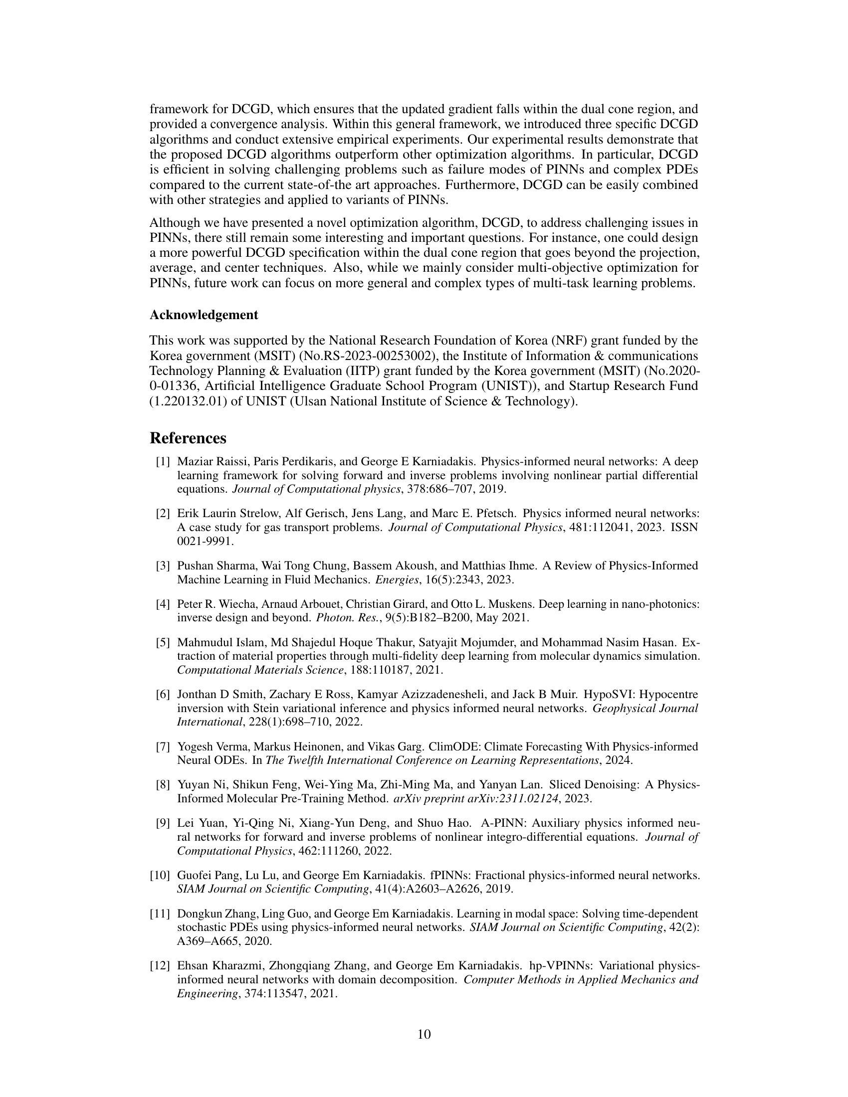
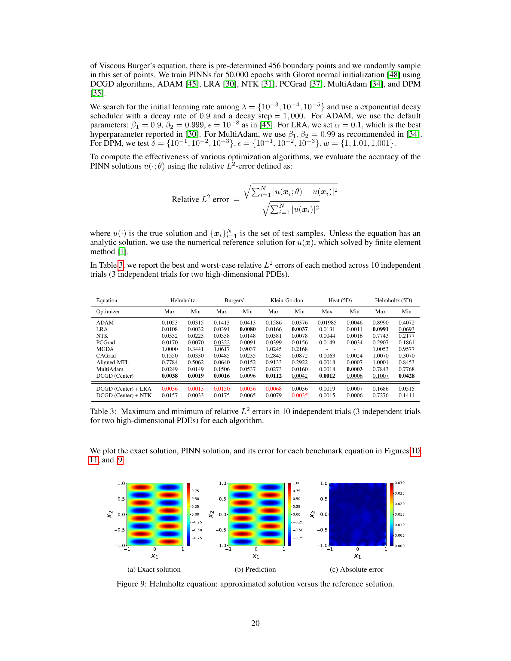
🔼 This table presents the relative L2 errors achieved by the Dual Cone Gradient Descent (DCGD) method and a baseline method for three different equations: the Chaotic Kuramoto-Sivashinsky (KS) equation, the Convection equation, and the Volterra integral differential equations (IDEs). The results demonstrate that DCGD significantly improves accuracy across all three equations compared to the baseline method, highlighting its effectiveness in solving complex PDEs.
read the caption
Table 2: Relative L2 errors for DCGD (Center) on Chaotic KS equation, Convection equation and Volterra IDEs.

🔼 This table presents the mean and standard deviation of the relative L2 error for various optimization algorithms across three benchmark PDEs (Helmholtz, Burgers, Klein-Gordon) and two high-dimensional PDEs (5D Heat, 3D Helmholtz). The results are based on 10 independent trials (3 for high-dimensional PDEs). A ‘-’ indicates that the optimizer failed to converge for that specific PDE.
read the caption
Table 1: Average of relative L2 errors in 10 independent trials for each algorithm on three benchmark PDEs (3 independent trials for two high-dimensional PDEs). The value within the parenthesis indicates the standard deviation. '-' denotes that the optimizer failed to converge.
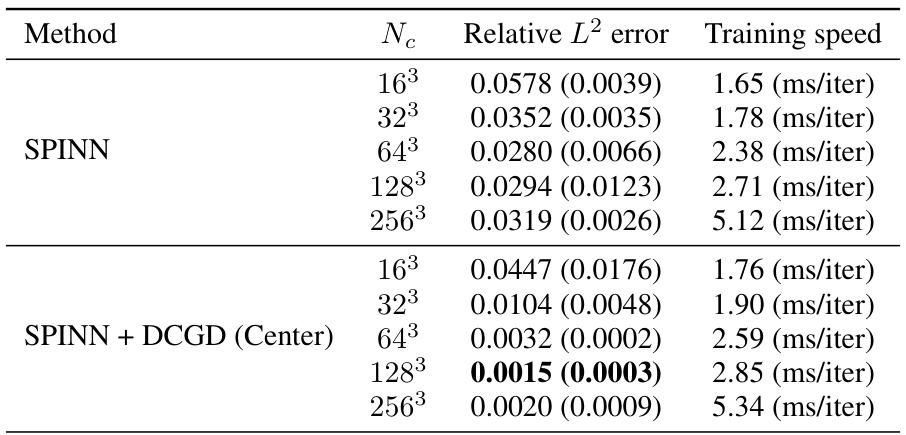
🔼 This table presents the mean and standard deviation of the relative L2 errors for various optimization algorithms applied to three benchmark PDEs (Helmholtz, Burgers, Klein-Gordon) and two high-dimensional PDEs (5D-Heat and 3D-Helmholtz). The results are averaged across 10 independent trials (3 for high-dimensional PDEs). The table highlights the performance of each optimizer, showing the mean and standard deviation of the relative L2 errors, including cases where the optimizer failed to converge.
read the caption
Table 1: Average of relative L2 errors in 10 independent trials for each algorithm on three benchmark PDEs (3 independent trials for two high-dimensional PDEs). The value within the parenthesis indicates the standard deviation. '-' denotes that the optimizer failed to converge.

🔼 This table presents the mean and standard deviation of the relative L2 error for various optimization algorithms applied to three benchmark partial differential equations (PDEs) and two high-dimensional PDEs. The relative L2 error measures the accuracy of the PINN solution trained by each optimizer. Lower values indicate better performance. The results are based on 10 independent trials for each algorithm, except for the two high-dimensional PDEs (Heat(5D) and Helmholtz(3D)) where only 3 independent trials were performed due to higher computational cost. The table helps to compare the performance of different optimization methods for solving PDEs using PINNs.
read the caption
Table 1: Average of relative L2 errors in 10 independent trials for each algorithm on three benchmark PDEs (3 independent trials for two high-dimensional PDEs). The value within the parenthesis indicates the standard deviation. '-' denotes that the optimizer failed to converge.

🔼 This table compares the performance of different optimization algorithms on three benchmark partial differential equations (PDEs) and two high-dimensional PDEs. The algorithms are evaluated using the average relative L2 error across 10 independent trials (3 trials for high-dimensional problems). Lower error values indicate better performance. The standard deviation of the error is also provided.
read the caption
Table 1: Average of relative L2 errors in 10 independent trials for each algorithm on three benchmark PDEs (3 independent trials for two high-dimensional PDEs). The value within the parenthesis indicates the standard deviation. '-' denotes that the optimizer failed to converge.
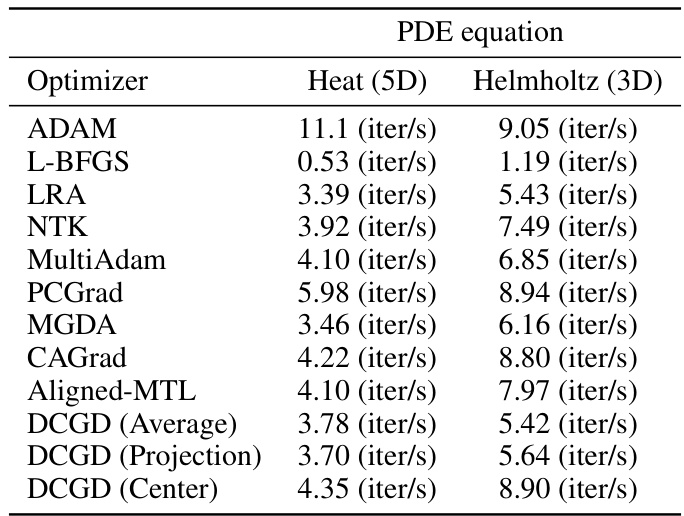
🔼 This table presents the performance comparison of different optimization algorithms for solving three benchmark partial differential equations (PDEs): Helmholtz, Burgers’, and Klein-Gordon, along with two high-dimensional PDEs (5D Heat and 3D Helmholtz). The results are averaged over 10 independent trials (3 for high-dimensional PDEs), showing the mean relative L2 error and its standard deviation for each algorithm. The table highlights the superior performance of DCGD, particularly when compared to commonly used optimizers like ADAM.
read the caption
Table 1: Average of relative L2 errors in 10 independent trials for each algorithm on three benchmark PDEs (3 independent trials for two high-dimensional PDEs). The value within the parenthesis indicates the standard deviation. '-' denotes that the optimizer failed to converge.
Full paper#


