TL;DR#
Traditional recurrent and Transformer models struggle with real-world time-series data due to high computational costs and difficulties handling irregularly sampled data or long-range dependencies. Neural ODE models offer an improvement for irregularly sampled data, but still struggle with long sequences. Existing methods, such as neural ODE and Transformer models, often exhibit high computational costs, especially when dealing with long sequences.
This paper introduces Rough Transformers, a novel approach that leverages path signatures for continuous-time representation of time series. The proposed model uses a multi-view signature attention mechanism that extracts both local and global dependencies in the data efficiently. Experimental results demonstrate that Rough Transformers outperform state-of-the-art methods on several tasks, achieving substantial computational savings while maintaining accuracy and robustness to irregular sampling.
Key Takeaways#
Why does it matter?#
This paper is crucial for researchers working with time-series data, especially those dealing with long, irregularly sampled sequences. Its introduction of Rough Transformers offers a novel approach to continuous-time sequence modeling, addressing the computational limitations of existing methods. This opens new avenues for research in various domains, including healthcare, finance, and biology. The improved efficiency and robustness of the proposed method will significantly benefit researchers working with large datasets and irregular sampling patterns. The method’s proven ability to capture both local and global dependencies in the data has great potential for impacting related research in various domains.
Visual Insights#

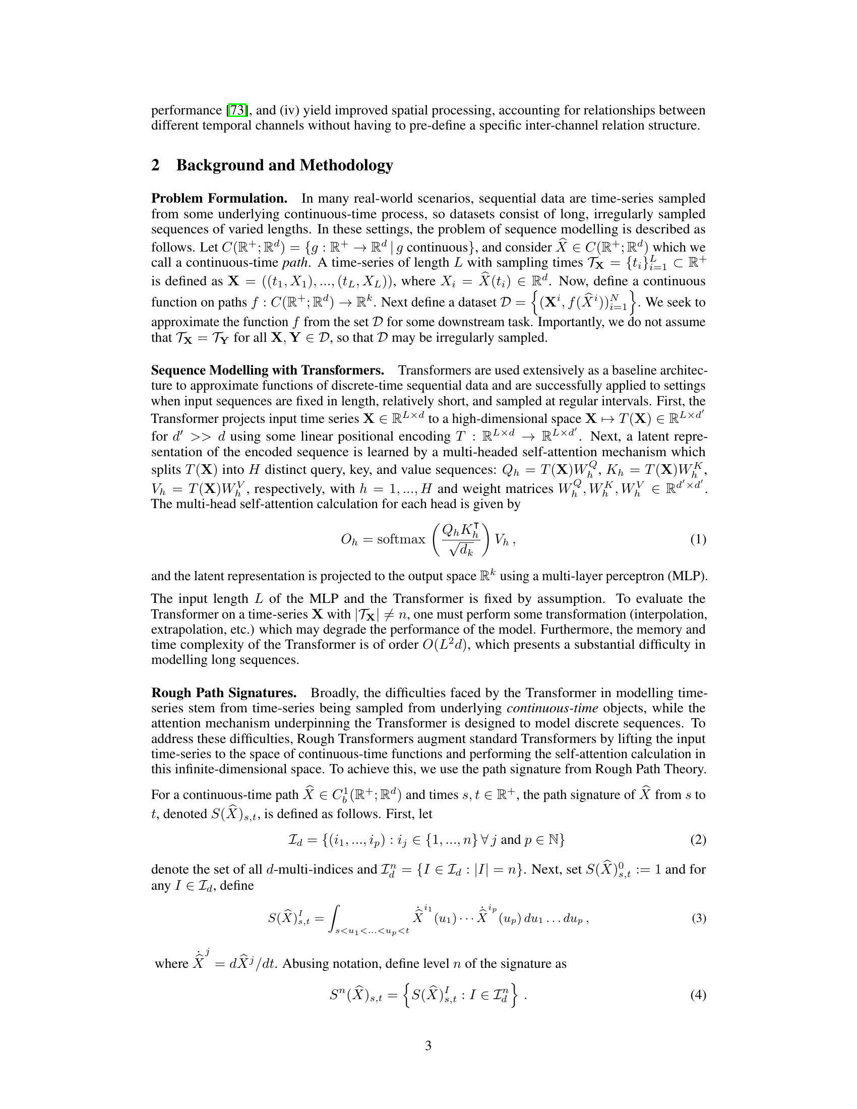
🔼 This figure illustrates the concept of a multi-view signature, a key component of the Rough Transformer architecture. It shows how an irregularly sampled continuous-time path (represented by the black curve with red x’s marking sample points) is transformed into a multi-view signature. This transformation involves two steps: 1) Linear interpolation of the irregularly sampled path to create a continuous representation, 2) Computation of both local (blue) and global (green) signatures of the interpolated path. These local and global signatures capture both local and global dependencies in the input time-series. Finally, the local and global signatures are concatenated to form the multi-view signature, which is then used as input to the Rough Transformer.
read the caption
Figure 1: A representation of the multi-view signature. The continuous-time path is irregularly sampled at points marked with a red x. The local and global signatures of a linear interpolation of these points are computed and concatenated to form the multi-view signature. The multi-view signature transform consists of multi-view signatures.
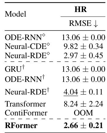
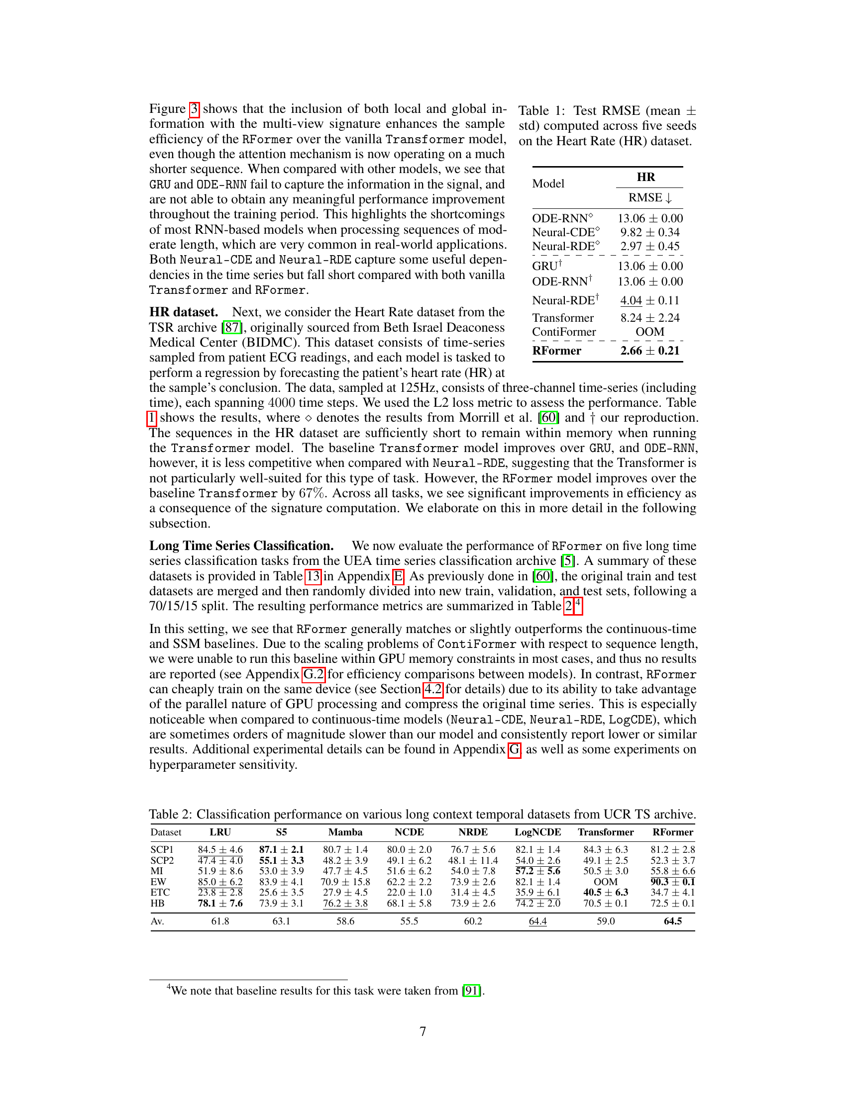
🔼 This table presents the test root mean squared error (RMSE) results for different models on the Heart Rate dataset. The RMSE is a measure of the average difference between predicted and actual heart rates. Lower RMSE values indicate better performance. The results are averaged across five separate trials (seeds) to provide a more robust estimate of model performance. The models compared include ODE-RNN, Neural-CDE, Neural-RDE, GRU, a standard Transformer model, ContiFormer, and the proposed Rough Transformer (RFormer). The plus sign (+) in Neural-RDE+ indicates the authors’ own reproduction of a result from another paper. ‘OOM’ stands for ‘out of memory’ and indicates that the ContiFormer model was unable to run on the given dataset due to memory limitations. The table highlights that RFormer achieves the lowest RMSE value, signifying superior performance.
read the caption
Table 1: Test RMSE (mean ± std) computed across five seeds on the Heart Rate (HR) dataset.
In-depth insights#
Rough Path Signatures#
Rough path signatures offer a powerful mathematical framework for representing and analyzing complex, irregular data, particularly time series. Their key advantage lies in their robustness to noise and irregular sampling, making them well-suited for real-world applications where data is often messy and incomplete. The path signature is a functional, capturing the essential features of a path by encoding its multi-scale dependencies in a way that is invariant to time reparameterization. This invariance simplifies computation and enhances the model’s ability to learn underlying dynamics from diverse sampling schemes. By representing paths as infinite series of iterated integrals, rough path theory allows for the approximation of continuous functions with linear functionals, significantly reducing computational complexity compared to traditional methods. Furthermore, the use of truncated signatures effectively controls the dimensionality of the resulting features. The multi-scale nature of the signature captures both local and global features within the data, providing a richer representation than simpler methods. Although computationally intensive, particularly for high dimensional data, techniques like log-signatures or randomized signatures can mitigate these issues.
Multi-view Attention#
The concept of “Multi-view Attention” in the context of time-series analysis using path signatures is a novel approach to capture both local and global dependencies within data. It leverages the inherent multi-scale nature of path signatures by incorporating both local and global views. The local view focuses on short-term, fine-grained dependencies, offering a type of convolutional filtering capability. The global view concentrates on long-range, holistic relationships, providing a more comprehensive contextual understanding. By concatenating these views, the model gains a richer, more complete understanding of the input data. This combined approach enhances robustness to irregular sampling frequencies and variations in sequence length. The effectiveness stems from the ability to represent continuous-time data efficiently while maintaining crucial local and global context, leading to potentially improved performance and reduced computational costs in downstream tasks.
Computational Efficiency#
The heading ‘Computational Efficiency’ likely discusses how the proposed method, Rough Transformers, reduces computational costs compared to existing approaches like vanilla Transformers and Neural ODEs. The core argument centers on reducing the quadratic time complexity (O(L²d)) of standard Transformers to a significantly lower complexity. This improvement is achieved by operating on compressed continuous-time representations of input sequences via path signatures, thereby reducing the effective sequence length. The authors may present empirical evidence of this reduced computational cost, showing speedups in training time and improved memory efficiency, particularly for long sequences. The methodology likely avoids costly numerical solvers needed by Neural ODEs, and pre-computable signature features further enhance efficiency. The discussion might also contrast the computational scaling characteristics of various models, emphasizing the superiority of Rough Transformers in handling high-dimensional and long sequences. Overall, this section aims to highlight the practical advantages of Rough Transformers by demonstrating their superior computational performance, thereby making them suitable for large-scale real-world applications.
Irregular Time Series#
Irregular time series pose a significant challenge in machine learning due to their non-uniform sampling intervals, making traditional methods like recurrent neural networks struggle. The absence of a fixed time step disrupts the temporal dynamics assumed by these models. Addressing this requires novel approaches that can effectively capture the complex relationships in data with varying time gaps between observations. Path signatures provide a powerful tool here by encoding the continuous-time nature of the underlying process. By converting irregularly sampled data to continuous-time representations via path signatures, the Rough Transformer avoids the drawbacks of relying solely on discrete-time input, offering robustness to variations in sampling frequency and length of input sequences. This enables more effective learning of long-range dependencies, even in scenarios with non-uniformly sampled or missing data. The performance gains are achieved without the computational complexities associated with traditional methods which need to solve ODEs numerically.
Future Research#
Future research directions stemming from this Rough Transformer work could explore several promising avenues. Extending the model to handle even higher-dimensional data is crucial, perhaps by leveraging techniques like log-signatures or randomized projections. Investigating the model’s robustness to noise and outliers in real-world scenarios warrants further attention. Developing a theoretical framework to better understand the model’s capacity for capturing long-range dependencies and its relationship to the path signature’s properties would be valuable. The model’s performance with different types of continuous-time processes and the impact of signature truncation on accuracy require additional investigation. Exploring applications in other domains beyond those initially explored in the paper is also warranted. Finally, comparative analyses against other state-of-the-art continuous-time models should be conducted on a wider range of datasets to establish clear performance benchmarks and highlight the strengths and limitations of this new approach.
More visual insights#
More on figures

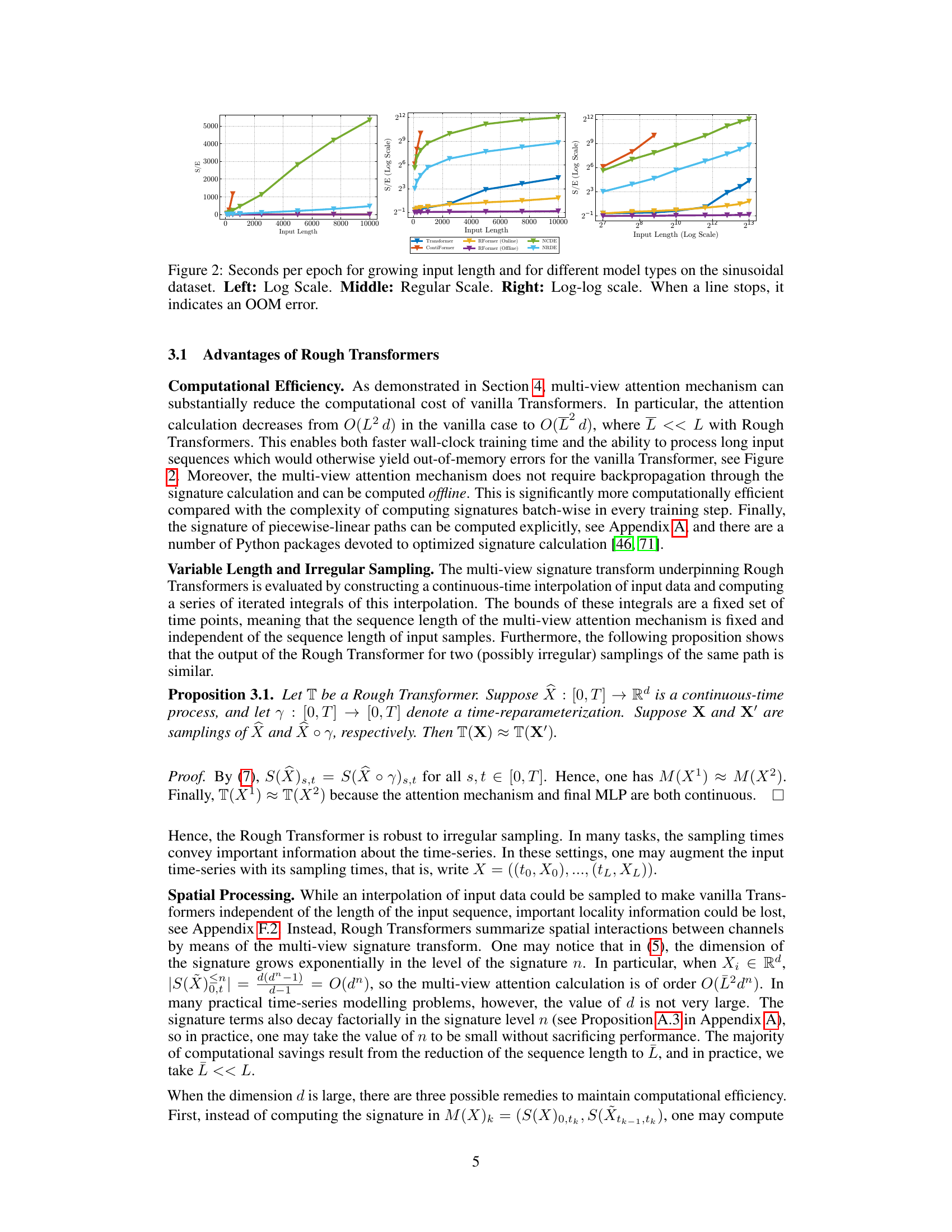
🔼 This figure compares the training time (seconds per epoch) of various models on a sinusoidal dataset as the input sequence length increases. The x-axis represents input length, and the y-axis shows seconds per epoch. The three subplots show the data using different scales: log scale, regular scale, and log-log scale. The different colored lines represent different models (Transformer, ContiFormer, Rough Transformer (Online and Offline), Neural CDE, Neural RDE). When a line stops, it means that the model ran out of memory (OOM). The figure demonstrates the superior computational efficiency of the Rough Transformer, particularly as the sequence length grows.
read the caption
Figure 2: Seconds per epoch for growing input length and for different model types on the sinusoidal dataset. Left: Log Scale. Middle: Regular Scale. Right: Log-log scale. When a line stops, it indicates an OOM error.

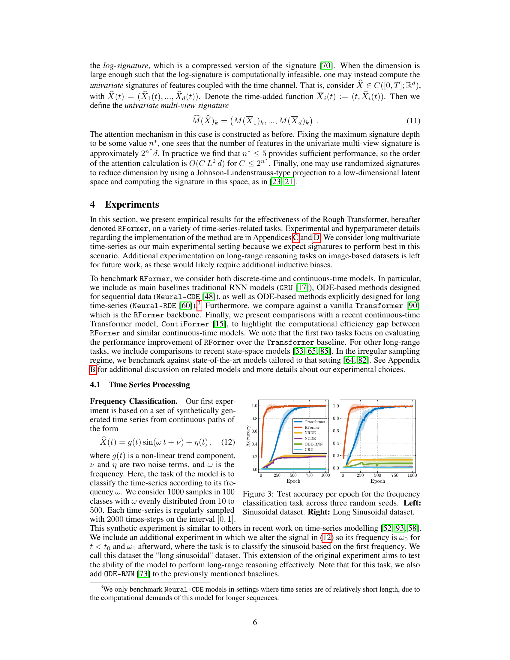
🔼 This figure shows the test accuracy per epoch for a frequency classification task. The task is performed on two datasets: a standard sinusoidal dataset and a more challenging ’long sinusoidal’ dataset. The figure compares the performance of several models: Transformer, RFormer, Neural ODE (NRDE), Neural Controlled Differential Equation (NCDE), ODE-RNN, and GRU. The plots illustrate the learning curves across three different random seeds, demonstrating the relative performance and convergence speed of each model on both datasets. The results show that the Rough Transformer (RFormer) outperforms other models in accuracy and convergence speed, particularly on the more challenging ’long sinusoidal’ dataset.
read the caption
Figure 3: Test accuracy per epoch for the frequency classification task across three random seeds. Left: Sinusoidal dataset. Right: Long Sinusoidal dataset.
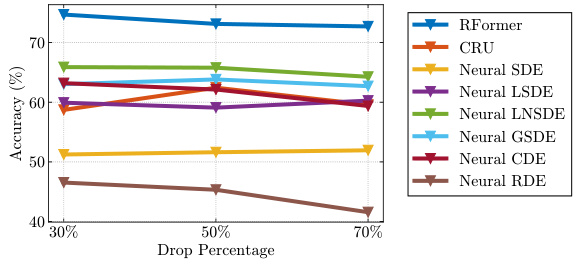
🔼 This figure shows the average performance of various models (RFormer, CRU, Neural SDE, Neural LSDE, Neural LNSDE, Neural GSDE, Neural CDE, Neural RDE) on 15 univariate datasets from the UEA Time Series archive under different data drop percentages (30%, 50%, 70%). The x-axis represents the data drop percentage, and the y-axis represents the accuracy. The figure demonstrates the robustness of RFormer to irregular sampling, maintaining relatively high accuracy even with significant data loss compared to other models.
read the caption
Figure 4: Average performance of all models on the 15 univariate datasets from the UEA Time Series archive under different degrees of data drop.

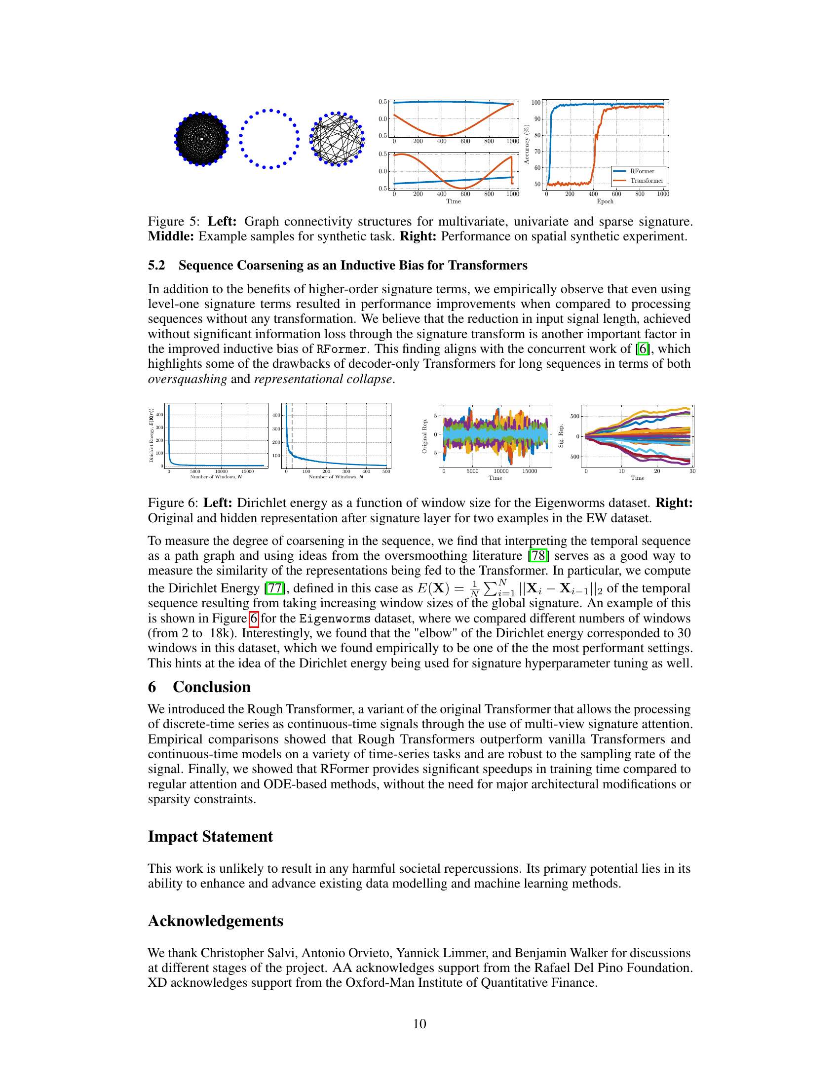
🔼 This figure demonstrates the spatial processing capabilities of the Rough Transformer. The left panel shows different graph structures representing the relationships between channels processed by the different signature types: multivariate, univariate, and sparse. The middle panel displays example samples from the synthetic experiment designed to evaluate spatial processing. The right panel shows the performance comparison between the Rough Transformer and a vanilla Transformer on the synthetic spatial task, highlighting the Rough Transformer’s superior sample efficiency and accuracy.
read the caption
Figure 5: Left: Graph connectivity structures for multivariate, univariate and sparse signature. Middle: Example samples for synthetic task. Right: Performance on spatial synthetic experiment.

🔼 This figure shows the impact of different window sizes on the Eigenworms dataset. The left panel shows a plot of the Dirichlet energy against the number of windows used for the global signature. The Dirichlet energy measures the smoothness of the representation. The right panel shows the original and compressed representations of two examples from the dataset after the signature layer. The compressed representations show that the signature transform effectively captures the essential information while reducing the dimensionality of the data.
read the caption
Figure 6: Left: Dirichlet energy as a function of window size for the Eigenworms dataset. Right: Original and hidden representation after signature layer for two examples in the EW dataset.

🔼 This figure shows the ablation study of the multi-view signature on the sinusoidal datasets. It compares the performance of using both global and local components of the signature against using only one of them. The left panel shows the results for the standard sinusoidal dataset, while the right panel presents the results for the long sinusoidal dataset. The results indicate that using both global and local components generally leads to better performance than using only one type of component. This highlights the importance of considering both local and global dependencies for accurate and efficient time series modeling.
read the caption
Figure 7: Ablation of local and local components of the multi-view signature for the sinusoidal datasets. Left: Sinusoidal dataset. Right: Long Sinusoidal dataset.
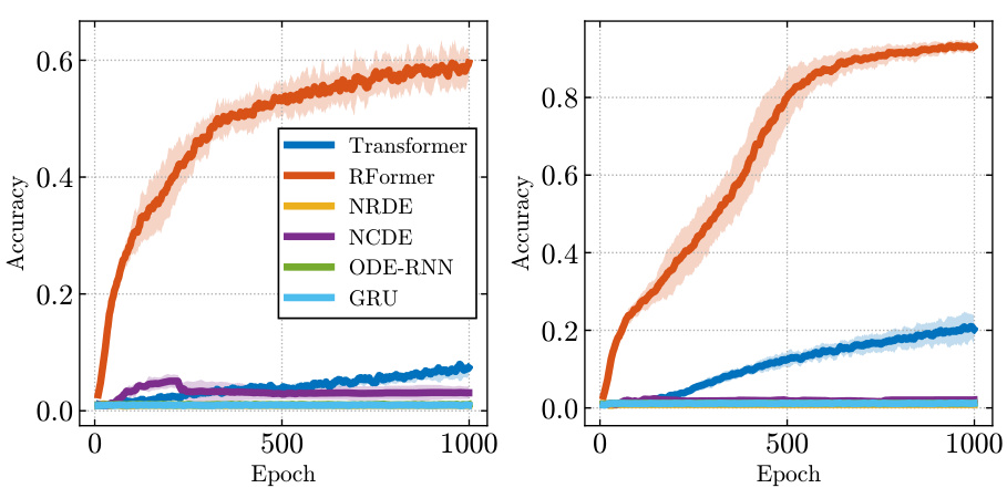
🔼 This figure shows the test accuracy per epoch for a frequency classification task using different models. Two datasets were used: a standard sinusoidal dataset and a ’long sinusoidal’ dataset. The ’long sinusoidal’ dataset is more complex, featuring a change in frequency midway through the time series, thus challenging the models’ ability to capture long-range dependencies. The results are averaged over three random seeds to show variability.
read the caption
Figure 3: Test accuracy per epoch for the frequency classification task across three random seeds. Left: Sinusoidal dataset. Right: Long Sinusoidal dataset.

🔼 This figure compares the training time (seconds per epoch) of different models on a sinusoidal dataset as the input sequence length increases. The x-axis represents the input sequence length, and the y-axis shows the seconds per epoch. Three subplots are provided: one with a logarithmic scale on both axes, one with a linear scale on the y-axis, and one with a logarithmic scale on the x-axis. The different colored lines represent different models: Transformer, ContiFormer, Rough Transformer (online), and Rough Transformer (offline). When a line abruptly ends, it indicates that the model ran out of memory (OOM). This figure highlights the computational efficiency of Rough Transformers, especially compared with the other models.
read the caption
Figure 2: Seconds per epoch for growing input length and for different model types on the sinusoidal dataset. Left: Log Scale. Middle: Regular Scale. Right: Log-log scale. When a line stops, it indicates an OOM error.
More on tables

🔼 This table presents the classification performance of different models on several long temporal datasets from the UCR Time Series Classification Archive. The datasets vary in characteristics like sequence length, number of classes, and dimensionality. The models compared include traditional machine learning methods like GRU, Neural CDE, Neural RDE, and LogCDE, as well as the vanilla Transformer and the proposed Rough Transformer (RFormer). The results show the average accuracy of each model across multiple runs, highlighting RFormer’s competitive performance and efficiency.
read the caption
Table 2: Classification performance on various long context temporal datasets from UCR TS archive.
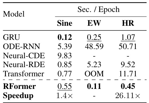
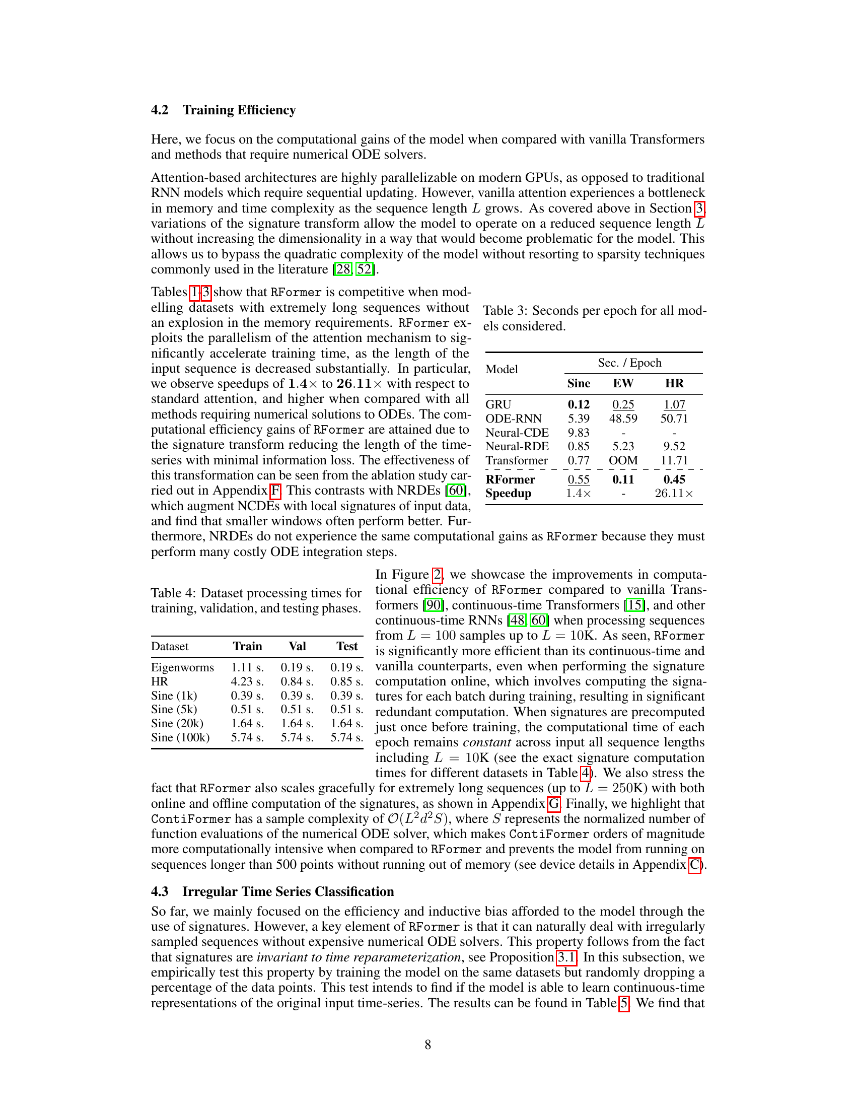
🔼 This table presents the training efficiency (seconds per epoch) for various models considered in the paper. It compares the Rough Transformer (RFormer) against several baseline models, including GRU, ODE-RNN, Neural-CDE, Neural-RDE, and the standard Transformer. The results highlight the significant computational advantages of RFormer, especially when dealing with the Heart Rate dataset.
read the caption
Table 3: Seconds per epoch for all models considered.
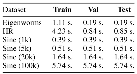
🔼 This table presents the time taken (in seconds) to process each dataset during the training, validation, and testing phases. The datasets include Eigenworms, HR (Heart Rate), and Sine wave datasets with varying lengths (1k, 5k, 20k, 100k samples). The table shows the computational efficiency of the Rough Transformer on datasets of various sizes.
read the caption
Table 4: Dataset processing times for training, validation, and testing phases.
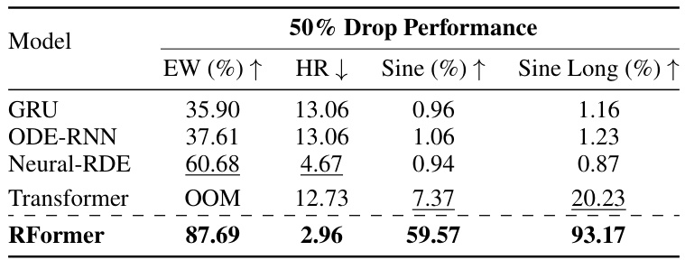
🔼 This table presents the performance of various models (GRU, ODE-RNN, Neural-RDE, Transformer, and RFormer) on different tasks (EW, HR, Sine, Sine Long) when 50% of the data points are randomly dropped per epoch. It demonstrates the robustness of the RFormer model to irregular sampling, showing consistent superior performance compared to other models, even with significant data loss.
read the caption
Table 5: Performance of all models under a random 50% drop in datapoints per epoch.
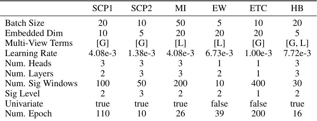
🔼 This table lists the hyperparameters used in the experiments reported in Table 2 of the paper. It shows the batch size, embedding dimension, multi-view terms (using global [G] or local [L] signatures, or a combination of both), learning rate, number of attention heads, number of layers, number of signature windows, signature level, whether univariate signatures were used, and the number of training epochs for six different datasets: SCP1, SCP2, MI, EW, ETC, and HB.
read the caption
Table 6: Hyperparameters used for Table 2, where G and L refer to the Global and Local signature components, respectively.

🔼 This table shows the hyperparameters used for validation on the remaining datasets after hyperparameter tuning on the sinusoidal dataset. It details the learning rate, number of windows used in the multi-view signature transform, signature depth, type of signature used (Multi-view or Local), and whether univariate or multivariate signatures were employed for each dataset (Sinusoidal, HR).
read the caption
Table 7: Hyperparameters validation on remaining datasets.
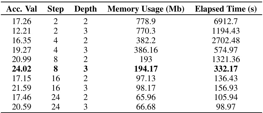
🔼 This table presents the validation accuracy results for different hyperparameter settings (Step and Depth) of the Neural-RDE model on the sinusoidal dataset. It shows the trade-off between model complexity (memory usage) and performance (accuracy) with varying step and depth values, which are crucial for tuning the model.
read the caption
Table 8: Validation accuracy on the sinusoidal dataset.
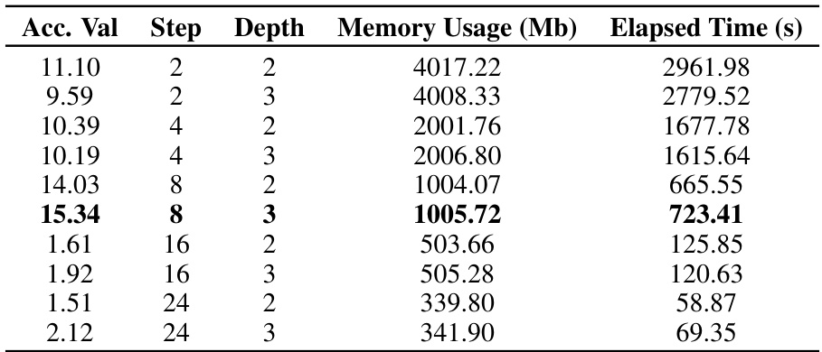
🔼 This table presents the validation accuracy results for the long sinusoidal dataset. It shows the accuracy achieved by the model with different hyperparameter settings (Step and Depth) of the Neural RDE model. Each row represents a different configuration, showing the resulting validation accuracy, memory usage, and elapsed time.
read the caption
Table 9: Validation accuracy on the long sinusoidal dataset.
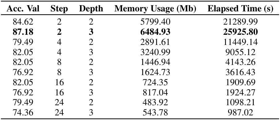
🔼 This table presents the validation accuracy achieved by the Rough Transformer model on the EigenWorms (EW) dataset. It shows the accuracy for different combinations of ‘Step’ and ‘Depth’ parameters within the multi-view signature transform. The memory usage (in MB) and elapsed training time (in seconds) are also reported for each configuration.
read the caption
Table 10: Validation accuracy on the EW dataset.

🔼 This table presents the test root mean squared error (RMSE) results for different models on the Heart Rate dataset. The RMSE is a measure of the models’ prediction accuracy, with lower values indicating better performance. The results are averaged across five random seeds to account for variability. Models include ODE-RNN, Neural-CDE, Neural-RDE, GRU, a standard Transformer, and the proposed Rough Transformer. The table shows that the Rough Transformer outperforms all other models except Neural-RDE, highlighting its effectiveness on this task.
read the caption
Table 1: Test RMSE (mean ± std) computed across five seeds on the Heart Rate (HR) dataset.

🔼 This table shows the validation loss for different hyperparameter settings (Step and Depth) of the Rough Transformer model on the LOB (Level 1) dataset with 1000 data points. The table details the validation loss, step size, depth, memory usage, and elapsed time for each hyperparameter configuration. It demonstrates the impact of these parameters on the model’s performance.
read the caption
Table 12: Validation loss on the LOB dataset (1K), included as an additional experiment in Appendix G.4.

🔼 This table presents a summary of the five long temporal datasets used for the long time-series classification experiments in the paper. For each dataset, the table shows the number of sequences, the length of each sequence, the number of classes, and the number of dimensions.
read the caption
Table 13: Summary of datasets used in the long time-series classification task.

🔼 This table compares the performance of Linear Interpolation + Vanilla Transformer against Rough Transformer with different signature levels (n) on two datasets: EigenWorms and HR. The ‘Improvement’ column shows the percentage increase in performance achieved by the Rough Transformer over the baseline method. The number in parentheses after the signature level indicates the level used for that particular dataset’s Rough Transformer result.
read the caption
Table 14: Comparative performance of different methods on datasets.

🔼 This table shows the performance of different models on the EigenWorms dataset under various data drop scenarios. The ‘Full’ column represents the performance on the complete dataset, while the other columns show performance when 30%, 50%, 70%, and 85% of the data is randomly dropped. The results highlight the robustness of the RFormer model compared to the Transformer model, especially under high data drop rates. The Transformer model fails to run at higher drop rates due to memory limitations, indicating its sensitivity to reduced data size.
read the caption
Table 15: Performance of models under various data drop scenarios for EW dataset.

🔼 This table shows the Root Mean Squared Error (RMSE) for the Heart Rate (HR) dataset under different percentages of randomly dropped data points (30%, 50%, 70%). It demonstrates the robustness of the Rough Transformer (RFormer) model, showing only a small increase in error even when a significant portion of the data is missing.
read the caption
Table 16: Performance consistency of RFormer under data drop scenarios for HR dataset.

🔼 This table presents the test accuracy of different models on the long sinusoidal dataset with 30% and 70% of data randomly dropped per epoch. The results are shown for epochs 100, 250, 500, and 1000, providing insights into model performance under different data scarcity conditions.
read the caption
Table 18: Epoch-wise performance under different data drop scenarios for the long sinusoidal dataset

🔼 This table shows the test accuracy of different models at various epochs (100, 250, 500, 1000) under different data drop scenarios (30% and 70%). The results are based on the long sinusoidal dataset. It highlights the model’s performance under data scarcity.
read the caption
Table 18: Epoch-wise performance under different data drop scenarios for the long sinusoidal dataset.
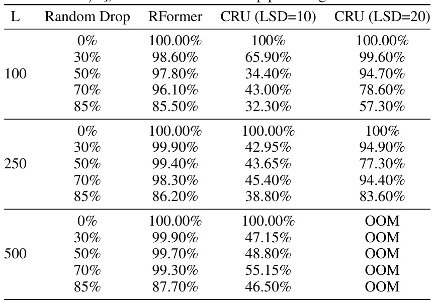
🔼 This table compares the performance of RFormer and CRU models on an irregularly sampled synthetic dataset with varying random drop percentages (0%, 30%, 50%, 70%, and 85%). The results show the accuracy of each model for different sequence lengths (100, 250, and 500) under different data drop scenarios, highlighting the robustness of RFormer to irregular sampling.
read the caption
Table 19: Comparison of RFormer and CRU (two best and simplest performing instances [Num.basis/Bandwidth= 20/3]) at different random drop percentages.
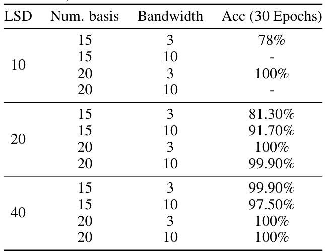
🔼 This table presents the hyperparameters used for the CRU model in the experiments with L=100. It shows different combinations of latent state dimension (LSD), number of basis matrices (Num. basis), and bandwidth, and reports the accuracy achieved after 30 epochs of training for each hyperparameter configuration.
read the caption
Table 20: CRU's hyperparameters (L = 100) (latent state dimension (LSD), number of basis matrices (Num.basis), and their bandwidth).

🔼 This table presents the training time (seconds per epoch) for various sequence lengths (from 100 to 10,000) using different models: NRDE, NCDE, GRU, CRU, ContiFormer, Transformer, and RFormer (with online and offline signature computation). It demonstrates the computational efficiency of the Rough Transformer, especially as sequence length increases, where other models experience out-of-memory (OOM) errors or significant slowdowns.
read the caption
Table 21: Seconds per epoch for growing input length and for different model types on the sinusoidal dataset.

🔼 This table presents the computational efficiency of various time series models (NRDE, NCDE, GRU, CRU, Contiformer, Transformer, RFormer(Online), RFormer(Offline)) for different input sequence lengths (L=100, L=250, L=500, L=1000, L=2500, L=5000, L=7.5k, L=10k). It shows the time taken per epoch (seconds) for each model as the input length increases. This is a key result highlighting the computational advantage of the proposed Rough Transformer model (RFormer) over other methods, especially for longer sequences.
read the caption
Table 21: Seconds per epoch for growing input length and for different model types on the sinusoidal dataset.

🔼 This table presents the processing times for different sequence lengths (sizes) on the sinusoidal dataset. It shows how the time required for processing increases as the length of the sequence increases. The times are given in seconds.
read the caption
Table 23: Processing times for different sizes on the sinusoidal dataset.

🔼 This table compares the performance of ContiFormer (with 1 and 4 heads), Transformer (1 head), and RFormer (1 head) models on a sinusoidal classification task with input sequence length L=100. The results are shown for epochs 100, 250, and 500, highlighting the training progress and the relative performance of each model.
read the caption
Table 24: Model performance for L = 100.

🔼 This table presents the results of a time-to-cancellation prediction task on limit order book (LOB) data using different models. It shows the Root Mean Squared Error (RMSE) and seconds per epoch (S/E) for each model with two different context window sizes (1k and 20k). The RMSE is a measure of the prediction accuracy, while S/E reflects the computational efficiency. Lower RMSE values indicate better prediction accuracy, and lower S/E values indicate higher computational efficiency. The table highlights the performance of the Rough Transformer (RFormer) against several baselines, including traditional Recurrent Neural Networks (RNNs), Neural ODEs, and the vanilla Transformer.
read the caption
Table 25: Test RMSE (mean ± std) and average seconds per epoch (S/E), computed across five seeds on the LOB dataset, on a scale of 10-2.

🔼 This table presents a comparison of the Root Mean Squared Error (RMSE) achieved by three different models: RFormer, the standard Transformer, and the Neural Rough Differential Equation (NRDE) model. The RMSE is a common metric used to evaluate the accuracy of regression models, where a lower RMSE indicates better performance. This table likely shows the results on a specific task or dataset to demonstrate the relative performance improvements of the RFormer model.
read the caption
Table 26: RMSE comparison between RFormer, Transformer, and NRDE.
Full paper#


