TL;DR#
Noisy labels are a pervasive problem in real-world regression tasks, hindering the accuracy and reliability of models. Existing methods for handling noisy labels often struggle with continuous labels, which are common in regression problems. There’s also a lack of standardized benchmark datasets for evaluating these methods, making comparisons difficult.
This paper introduces ConFrag, a novel approach that addresses these challenges. ConFrag transforms regression data into contrasting fragmentation pairs, enabling the training of distinctive representations for selecting clean samples. The method uses a mixture of neighboring fragments to identify noisy labels and is evaluated on six new benchmark datasets. Experiments show that ConFrag significantly outperforms fourteen state-of-the-art baselines across various noise types, demonstrating robustness and improved accuracy. A new metric, ERR, is also proposed to better evaluate the performance of methods on datasets with varying noise levels.
Key Takeaways#
Why does it matter?#
This paper is crucial for researchers working with noisy data in regression tasks. It introduces a novel method, showing consistent improvement over existing baselines and offering a new approach to handle label noise effectively. The six new benchmark datasets created are a significant contribution, enabling researchers to compare methods rigorously. The proposed ERR metric also advances the evaluation of noisy label regression, improving future research.
Visual Insights#

🔼 This figure demonstrates the effect of contrastive fragment pairing using t-SNE visualizations. Panel (a) shows how the method transforms some closed-set noisy samples into open-set noisy samples, which are less harmful. Panel (b) shows that open-set noise leads to lower errors. Panel (c) compares the performance of contrastive fragment pairing against using all fragments together, showing that the contrastive approach is more effective.
read the caption
Figure 1: (a) An example of t-SNE illustration of contrastive fragment pairing. The data with label noise are grouped into six fragments (f ∈ [1-6]) and formed into three contrastive pairs (f∈ [1, 4], [2, 5], [3, 6]). Contrastive fragment pairing transforms some of closed-set noise (whose ground truth is within the target label set) into open-set noise (whose ground truth is not within the label set). For example, in the [1,4] figure, label noise whose ground truth fragment is either 1 or 4 is closed-set noise, and the others are open-set noise. The t-SNE illustration shows that learned features of open-set noises tend to reside outside the feature clusters of the clean samples. (b) The open-set noise is less harmful with much lower errors (MRAE) in the downstream regression. (c) The contrastive pairing ([1, 4], [2, 5], [3, 6]) is more effective than using all-fragments together ([1-6]), resulting in much lower MRAE scores. All experiments are based on IMDB-Clean-B with more details in Appendix G.4-G.5.
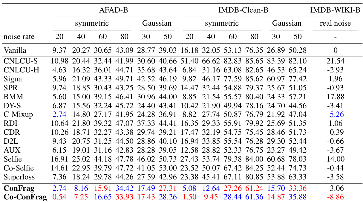
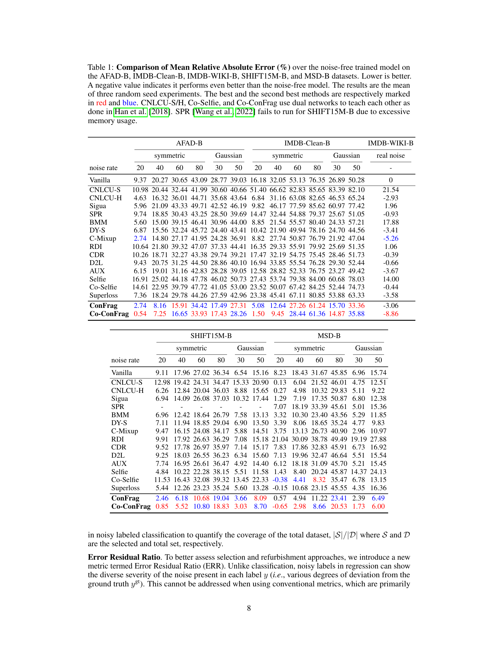
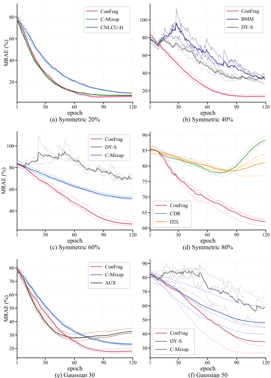
🔼 This table compares the performance of ConFrag and fourteen other state-of-the-art baselines on five benchmark datasets for noisy label regression. The Mean Relative Absolute Error (MRAE) is reported for various noise levels (symmetric and Gaussian noise). Lower MRAE indicates better performance. The table highlights the superior performance of ConFrag, especially when compared to baselines that do not explicitly address noisy labels. A negative MRAE value signifies superior performance to the noise-free model.
read the caption
Table 1: Comparison of Mean Relative Absolute Error (%) over the noise-free trained model on the AFAD-B, IMDB-Clean-B, IMDB-WIKI-B, SHIFT15M-B, and MSD-B datasets. Lower is better. A negative value indicates it performs even better than the noise-free model. The results are the mean of three random seed experiments. The best and the second best methods are respectively marked in red and blue. CNLCU-S/H, Co-Selfie, and Co-ConFrag use dual networks to teach each other as done in Han et al. [2018]. SPR [Wang et al., 2022] fails to run for SHIFT15M-B due to excessive memory usage.
In-depth insights#
Noisy Label Reg#
Noisy label regression tackles the challenges of training accurate models when the training data contains incorrect or unreliable labels. This is a pervasive issue in real-world applications where data acquisition is costly or time-consuming, leading to imperfect annotations. Techniques for addressing noisy labels often involve either modifying the loss function to down-weight noisy samples or attempting to identify and remove noisy data points. Methods may leverage data augmentation to generate more robust representations or incorporate regularization to prevent overfitting to the incorrect labels. The choice of technique depends on factors such as the type of noise, its prevalence, and the complexity of the model. Research in this area is actively exploring the use of deep learning and advanced statistical models to improve the robustness and accuracy of noisy label regression. Furthermore, evaluating and selecting the most suitable approach for a given dataset remains a challenge requiring careful consideration of the noise characteristics and model limitations. Creating benchmark datasets to evaluate noisy label regression methods is vital to advance the field and allow for fair comparisons between different techniques.
ConFrag Method#
The ConFrag method, designed for noisy label regression, leverages the inherent property of continuous ordered correlations in real-world data. It begins by dividing the data into contrastive fragment pairs, maximizing the distance between paired fragments in label space. This step is crucial, transforming some closed-set noise (noise within the target label range) into less harmful open-set noise. The method trains expert feature extractors on these pairs, generating distinctive representations which are less susceptible to overfitting. To further refine sample selection, ConFrag utilizes a mixture model incorporating neighboring fragments, leveraging neighborhood agreement to identify clean samples. This multi-expert approach improves robustness and generalizability. Finally, the method incorporates neighborhood jittering as a regularizer to avoid overfitting by expanding data coverage for each expert during training, resulting in improved model performance.
Benchmark Data#
The effectiveness of any novel approach in noisy label regression heavily relies on the quality and diversity of benchmark datasets used for evaluation. A robust benchmark should encompass diverse data domains, varying noise types and intensities, and ideally, real-world noisy labels reflecting the challenges faced in practical applications. Creating such a benchmark is crucial, as the absence of a standardized, well-curated benchmark hinders fair comparison and limits the generalizability of findings. The selection of datasets should be guided by the characteristics of the proposed method, ensuring that the datasets adequately challenge the algorithm’s strengths and weaknesses. For instance, a method focusing on continuous labels would benefit from datasets with intrinsically ordered correlations between labels and features, while a method designed for image-based regression should include datasets containing image data with noisy labels. Careful analysis of existing datasets is essential to identify and address potential biases or limitations before incorporating them into the benchmark. This includes checking for class imbalances, noise distribution patterns, and ensuring a representative range of sample complexities. Ultimately, a comprehensive benchmark ensures the rigorous evaluation of new methods, promoting advancement in the field by facilitating consistent and meaningful comparisons.
Future Research#
Future research directions stemming from this work could explore several promising avenues. Improving the scalability of the ConFrag framework is crucial, potentially through exploring more efficient Mixture of Experts (MoE) architectures or alternative sample selection methods. Investigating the impact of different fragmentation strategies and the optimal number of fragments (F) across diverse datasets would also be valuable. Developing a more robust and theoretically grounded method for neighborhood agreement could enhance sample selection accuracy. Further research could explore ConFrag’s application to other regression tasks and potentially other machine learning problems beyond noisy label scenarios. Finally, a comprehensive comparative analysis incorporating more state-of-the-art noisy label regression techniques and a broader range of noise types would solidify the findings and advance the understanding of noisy label regression.
ConFrag Limits#
The effectiveness of ConFrag hinges on several factors, creating potential limitations. The reliance on the Mixture of Experts (MoE) model introduces scalability challenges, particularly concerning memory and computational resources, especially as the number of fragments increases. This could restrict its applicability to datasets exceeding a certain size or complexity. The reliance on neighborhood agreement for clean sample selection might be sensitive to the density and distribution of the data. In sparsely populated regions of the feature space or with high levels of label noise, the algorithm’s accuracy in identifying clean samples may be compromised. Moreover, the performance of ConFrag is affected by the hyperparameters, such as the number of fragments and the jitter range. Careful tuning is necessary to obtain optimal results, which can be computationally expensive. Finally, while ConFrag shows robustness to several types of noise, its performance might degrade with entirely different noise distributions or complex noise patterns not considered in the experiments.
More visual insights#
More on figures

🔼 The figure illustrates the algorithm for contrastive fragment pairing. The dataset is first divided into fragments based on the continuous labels. Then, a graph is constructed where each fragment is a node, and the edge weight between nodes represents the distance between the closest samples of the fragments in the label space. Finally, the algorithm finds a perfect matching (a pairing of fragments) that maximizes the minimum edge weight, ensuring the selected pairs are maximally contrasting.
read the caption
Figure 2: The contrastive fragment pairing algorithm.
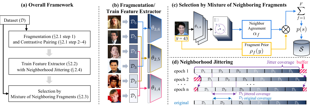
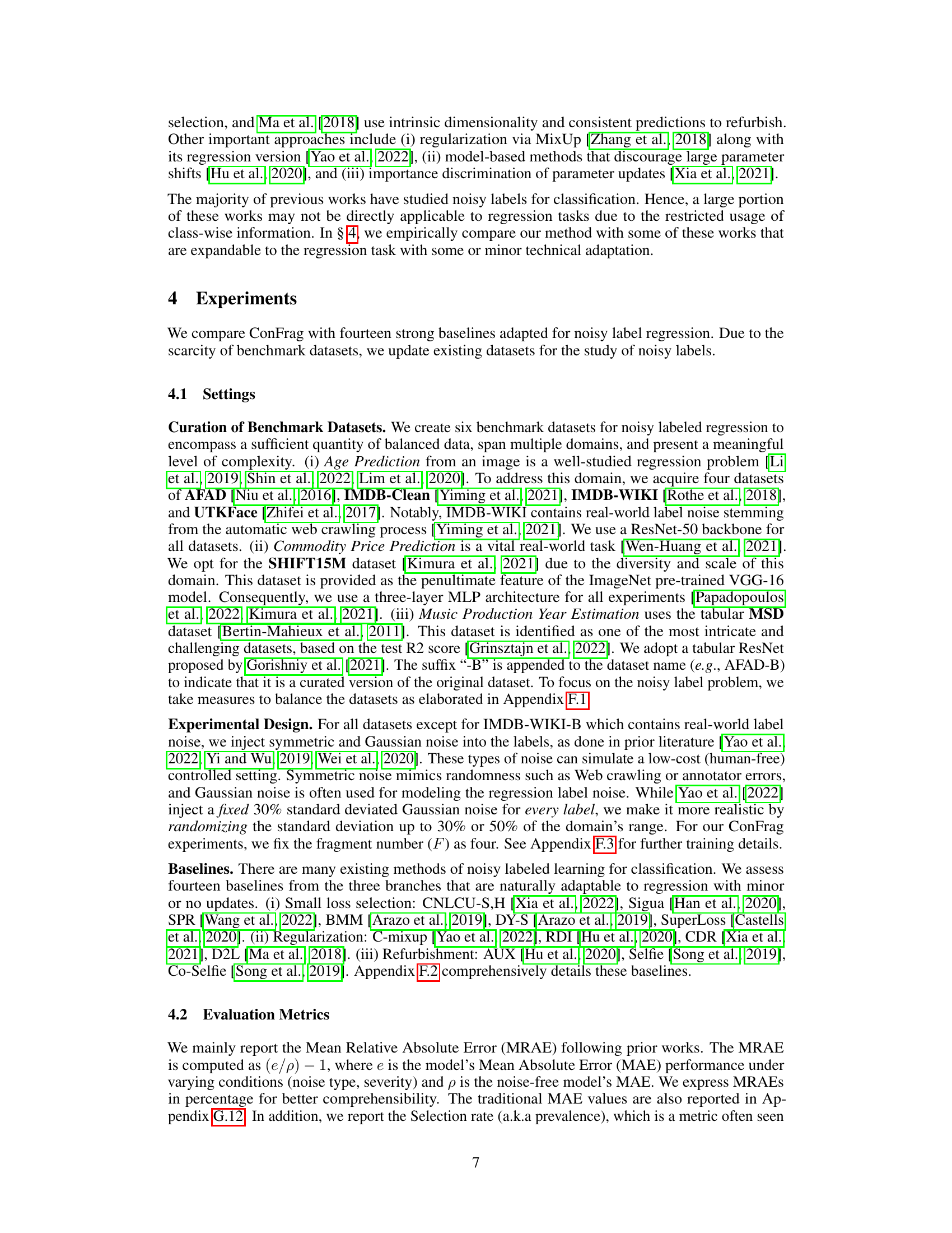
🔼 This figure illustrates the ConFrag framework, showing the steps involved in its process. (a) provides a high-level overview of the framework. (b) details the fragmentation of the continuous label space into contrastive fragment pairs and the subsequent training of feature extractors. (c) explains how sample selection is performed using a mixture of neighboring fragments. (d) demonstrates the concept of neighborhood jittering to enhance the selection process.
read the caption
Figure 3: Contrastive Fragmentation framework. (a) The overall sequential process of our framework. (b) Shows the fragmentation of the continuous label space to obtain contrasting fragment pairs (§ 2.1) and train feature extractors on them. (c) Sample Selection by Mixture of Neighboring Fragments obtains the selection probability in both prediction and representation perspectives (§ 2.3). (d) Illustration of Neighborhood Jittering (§ 2.4).

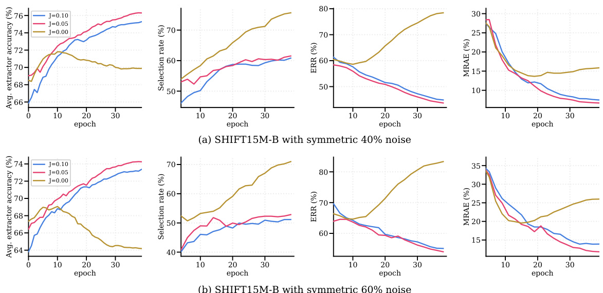
🔼 This figure shows the effects of neighborhood jittering regularization on the performance of feature extractors, sample selection, and regression. Panel (a) demonstrates that without jittering, feature extractors trained on noisy data tend to overfit, while jittering helps them generalize better. Panel (b) shows that the overfitting leads to higher selection rates and higher Error Residual Ratios (ERR), indicating poorer sample selection quality. Finally, panel (c) reveals that jittering regularization improves the final regression model’s performance.
read the caption
Figure 4: Jittering analysis. (a) When trained without jittering, feature extractors easily overfit the noisy training data (yellow-shaded region), while jittering-regularized feature extractors robustly learn from the noisy training data. (b) Overfitted feature extractors (yellow-shaded region) on noisy samples increase their likelihood, leading to a higher selection rate and ERR. It exhibits nearly twice higher ERR (a lower value is better). (c) Most importantly, jittering regularization improves performance in regression.

🔼 This figure compares the performance of ConFrag against five other strong baselines (CNLCU-H, BMM, DY-S, AUX, and Selfie) on the IMDB-Clean-B dataset. The comparison is based on three metrics: selection rate, error residual ratio (ERR), and mean relative absolute error (MRAE). The warm-up phase of training is excluded from the analysis. The figure shows that ConFrag achieves a better balance between selection rate, ERR, and MRAE compared to the other methods. Specifically, ConFrag demonstrates a lower ERR (indicating cleaner selected samples) and maintains a reasonably high selection rate, ultimately resulting in better regression performance (lower MRAE).
read the caption
Figure 5: Selection/ERR/MRAE comparison between ConFrag and strong baselines of CNLCU-H, BMM, DY-S, AUX and Selfie on IMDB-Clean-B. We exclude the performance during the warm-up.

🔼 This figure illustrates the ConFrag framework, showing the four main steps involved: (a) an overview of the entire process; (b) the fragmentation of the continuous label space into contrasting fragment pairs to train feature extractors; (c) sample selection based on both predictive and representational aspects using a mixture of neighboring fragments; and (d) the application of neighborhood jittering for regularization. Each step visually shows the data transformations and models used.
read the caption
Figure 3: Contrastive Fragmentation framework. (a) The overall sequential process of our framework. (b) Shows the fragmentation of the continuous label space to obtain contrasting fragment pairs (§ 2.1) and train feature extractors on them. (c) Sample Selection by Mixture of Neighboring Fragments obtains the selection probability in both prediction and representation perspectives (§ 2.3). (d) Illustration of Neighborhood Jittering (§ 2.4).

🔼 This figure shows the effect of contrastive fragment pairing using t-SNE visualization. It demonstrates how the method transforms some closed-set noise into open-set noise, resulting in lower errors. The contrastive pairing approach is shown to be more effective than using all fragments together.
read the caption
Figure 1: (a) An example of t-SNE illustration of contrastive fragment pairing. The data with label noise are grouped into six fragments (f ∈ [1-6]) and formed into three contrastive pairs (f∈ [1, 4], [2, 5], [3, 6]). Contrastive fragment pairing transforms some of closed-set noise (whose ground truth is within the target label set) into open-set noise (whose ground truth is not within the label set). For example, in the [1,4] figure, label noise whose ground truth fragment is either 1 or 4 is closed-set noise, and the others are open-set noise. The t-SNE illustration shows that learned features of open-set noises tend to reside outside the feature clusters of the clean samples. (b) The open-set noise is less harmful with much lower errors (MRAE) in the downstream regression. (c) The contrastive pairing ([1, 4], [2, 5], [3, 6]) is more effective than using all-fragments together ([1-6]), resulting in much lower MRAE scores. All experiments are based on IMDB-Clean-B with more details in Appendix G.4-G.5.

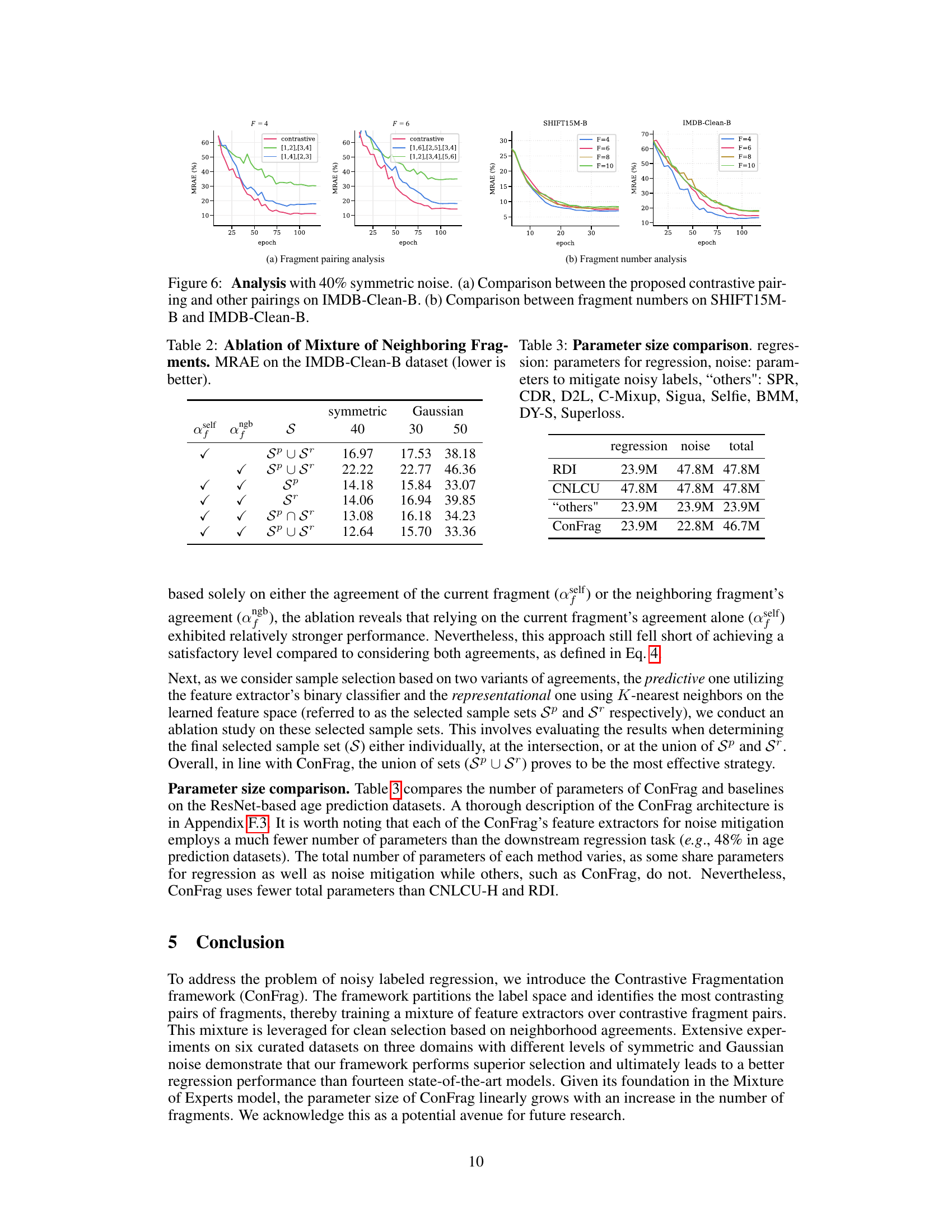
🔼 Figure 6 presents a comparison of the performance of contrastive fragment pairing against various alternative pairing strategies and different numbers of fragments. The left panel (a) focuses on the IMDB-Clean-B dataset and illustrates the superior performance of contrastive fragment pairing, showcasing its effectiveness in minimizing errors compared to using all fragments or other pairing methods. The right panel (b) explores the impact of varying the number of fragments on two datasets, SHIFT15M-B and IMDB-Clean-B, showing relatively stable performance on SHIFT15M-B but a decline on IMDB-Clean-B when using more fragments, likely due to overfitting.
read the caption
Figure 6: Analysis with 40% symmetric noise. (a) Comparison between the proposed contrastive pairing and other pairings on IMDB-Clean-B. (b) Comparison between fragment numbers on SHIFT15M-B and IMDB-Clean-B.

🔼 The figure shows two heatmaps visualizing the effects of random Gaussian noise injection on the label space. In (a), Gaussian noise is added with standard deviations randomly sampled from the range 1 to 30; in (b), the range is 1 to 50. The heatmaps depict the relationship between clean labels and their corresponding noisy labels, illustrating the variability and severity of the noise introduced. Darker colors represent a higher probability of a particular clean label being assigned a particular noisy label.
read the caption
Figure 9: Random Gaussian Noise. (a) Gaussian noise injected from the uniformly sampled random standard deviation between [1, 30]. (b) Gaussian noise injected from uniformly sampled random standard deviation between [1, 50].

🔼 The figure shows the training curves of selection rate, error residual ratio (ERR), and mean relative absolute error (MRAE) on the IMDB-Clean-B dataset with 40% symmetric noise using different numbers of fragments (F). It compares the performance of ConFrag with different fragment numbers (F = 4, 6, 8, 10) against the vanilla model. It demonstrates that ConFrag maintains stable performance across different fragment numbers, while the vanilla model’s performance degrades over time due to memorization of noisy samples.
read the caption
Figure 10: Fragment number analysis compares the Selection rate, ERR and MRAE on IMDB-Clean-B with symmetric 40% noise.
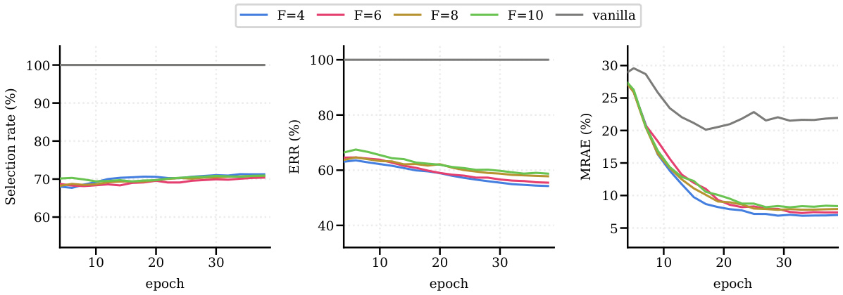
🔼 This figure shows the impact of varying the number of fragments (F) in the ConFrag model on three key metrics: Selection rate, Error Residual Ratio (ERR), and Mean Relative Absolute Error (MRAE). The experiment is performed on the IMDB-Clean-B dataset with 40% symmetric label noise. The results show how the performance changes across different values of F (4, 6, 8, 10), along with a comparison to a vanilla model (without ConFrag). Each line represents the trends of the three metrics over training epochs.
read the caption
Figure 10: Fragment number analysis compares the Selection rate, ERR and MRAE on IMDB-Clean-B with symmetric 40% noise.

🔼 The figure shows the effects of changing the hyperparameter K on the performance of the ConFrag model. The hyperparameter K controls the number of nearest neighbors considered when calculating neighborhood agreement for sample selection. The plots show selection rate, error residual ratio (ERR), and mean relative absolute error (MRAE) over training epochs for three different values of K (3, 5, and 7). The results indicate that there is an optimal value of K for balancing the trade-off between selecting many samples (high selection rate) and selecting primarily clean samples (low ERR and MRAE).
read the caption
Figure 12: Hyperparameter K analysis compares the Selection rate, ERR and MRAE on IMDB-Clean-B with symmetric 40% noise.

🔼 This figure shows the impact of varying the K-nearest neighbor parameter (K) on the performance of the ConFrag model. The three metrics (Selection Rate, ERR, and MRAE) are plotted against the training epoch for different values of K (3, 5, and 7). The Selection Rate represents the percentage of data points selected by the model as clean. ERR (Error Residual Ratio) reflects the ratio of error in the selected samples to the total error, while MRAE (Mean Relative Absolute Error) is a metric for regression performance. The plot illustrates how different values of K affect the model’s ability to select clean data and its overall performance.
read the caption
Figure 12: Hyperparameter K analysis compares the Selection rate, ERR and MRAE on IMDB-Clean-B with symmetric 40% noise.
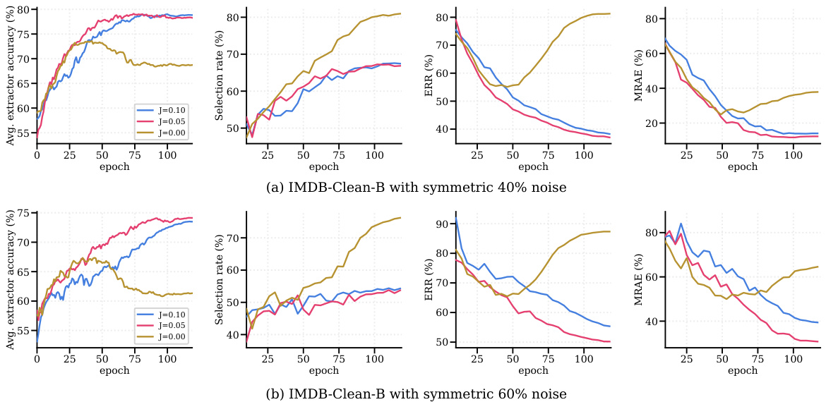
🔼 This figure demonstrates the effect of neighborhood jittering on feature extraction, sample selection, and regression performance. Panel (a) shows that without jittering, feature extractors overfit to noisy data, while jittering improves robustness. Panel (b) shows how overfitting leads to increased selection rates and error residual ratios (ERR). Finally, panel (c) highlights that jittering significantly improves regression performance.
read the caption
Figure 4: Jittering analysis. (a) When trained without jittering, feature extractors easily overfit the noisy training data (yellow-shaded region), while jittering-regularized feature extractors robustly learn from the noisy training data. (b) Overfitted feature extractors (yellow-shaded region) on noisy samples increase their likelihood, leading to a higher selection rate and ERR. It exhibits nearly twice higher ERR (a lower value is better). (c) Most importantly, jittering regularization improves performance in regression.
🔼 The figure shows the comparison of selection rate, error residual ratio (ERR), and mean relative absolute error (MRAE) on the IMDB-Clean-B dataset with 40% symmetric noise, across different numbers of fragments (F) used in ConFrag. The results illustrate how the performance metrics vary with different fragmentation schemes, providing insights into the optimal number of fragments for balancing model generalization and noise mitigation.
read the caption
Figure 10: Fragment number analysis compares the Selection rate, ERR and MRAE on IMDB-Clean-B with symmetric 40% noise.

🔼 This figure illustrates the ConFrag framework, showing the process of fragmenting the continuous label space into contrasting fragment pairs and training separate feature extractors on them. It then depicts the sample selection process using a mixture of neighboring fragments and the use of neighborhood jittering regularization to enhance the model’s performance and mitigate overfitting.
read the caption
Figure 3: Contrastive Fragmentation framework. (a) The overall sequential process of our framework. (b) Shows the fragmentation of the continuous label space to obtain contrasting fragment pairs (§ 2.1) and train feature extractors on them. (c) Sample Selection by Mixture of Neighboring Fragments obtains the selection probability in both prediction and representation perspectives (§ 2.3). (d) Illustration of Neighborhood Jittering (§ 2.4).
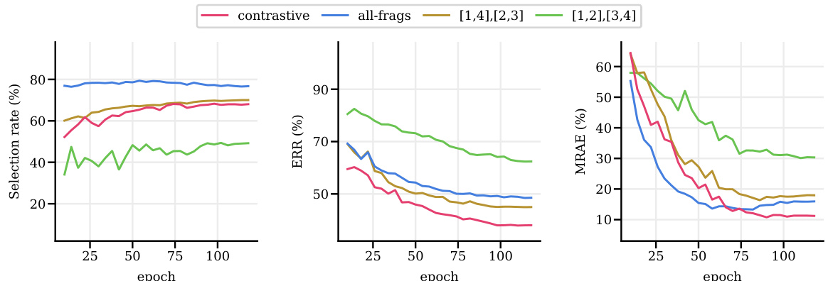
🔼 This figure shows a comparison of the selection rate, error residual ratio (ERR), and mean relative absolute error (MRAE) for different numbers of fragments (F) in the ConFrag model. The results are shown for the IMDB-Clean-B dataset with 40% symmetric noise. The plot illustrates how the model’s performance changes as the number of fragments is varied. The figure allows for a visual assessment of the impact of the hyperparameter F on the overall performance of the ConFrag framework.
read the caption
Figure 10: Fragment number analysis compares the Selection rate, ERR and MRAE on IMDB-Clean-B with symmetric 40% noise.
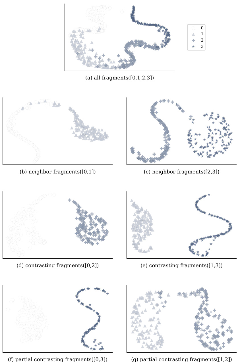
🔼 This figure illustrates the concept of contrastive fragment pairing using t-SNE visualizations. It shows how the proposed method transforms some closed-set noise (noise where the true label is within the selected fragments) into open-set noise (noise where the true label is outside the selected fragments). This transformation is beneficial because open-set noise is less detrimental to model performance. The figure also compares the effectiveness of contrastive pairing versus using all fragments together, demonstrating that contrastive pairing leads to improved downstream regression performance.
read the caption
Figure 1: (a) An example of t-SNE illustration of contrastive fragment pairing. The data with label noise are grouped into six fragments (f ∈ [1-6]) and formed into three contrastive pairs (f∈ [1, 4], [2, 5], [3, 6]). Contrastive fragment pairing transforms some of closed-set noise (whose ground truth is within the target label set) into open-set noise (whose ground truth is not within the label set). For example, in the [1,4] figure, label noise whose ground truth fragment is either 1 or 4 is closed-set noise, and the others are open-set noise. The t-SNE illustration shows that learned features of open-set noises tend to reside outside the feature clusters of the clean samples. (b) The open-set noise is less harmful with much lower errors (MRAE) in the downstream regression. (c) The contrastive pairing ([1, 4], [2, 5], [3, 6]) is more effective than using all-fragments together ([1-6]), resulting in much lower MRAE scores. All experiments are based on IMDB-Clean-B with more details in Appendix G.4-G.5.

🔼 This figure displays the result of injecting both closed-set and open-set noisy samples into the clean dataset, and how that affects selection rate, ERR, and MRAE. Closed-set noise is more harmful than open-set noise, because closed-set samples have labels that fall within the correct fragment’s boundaries, but are not correctly labeled. Open-set samples have labels outside of any correct fragment. The figure shows that the approach used is beneficial for reducing the effects of closed-set noise.
read the caption
Figure 19: Closed-set/open-set noise analysis displays the selection, ERR and MRAE when closed-set or open-set noisy samples are injected into the clean dataset. The experiments are based on IMDB-Clean-B.

🔼 This figure shows the effect of neighborhood jittering regularization on the performance of the ConFrag model. Panel (a) compares the average accuracy of feature extractors trained with and without jittering, showing that jittering prevents overfitting to noisy data. Panel (b) shows that overfitting leads to a higher selection rate and a much larger ERR (Error Residual Ratio). A lower ERR value indicates better performance. Finally, panel (c) demonstrates that jittering improves the regression performance of the model.
read the caption
Figure 4: Jittering analysis. (a) When trained without jittering, feature extractors easily overfit the noisy training data (yellow-shaded region), while jittering-regularized feature extractors robustly learn from the noisy training data. (b) Overfitted feature extractors (yellow-shaded region) on noisy samples increase their likelihood, leading to a higher selection rate and ERR. It exhibits nearly twice higher ERR (a lower value is better). (c) Most importantly, jittering regularization improves performance in regression.

🔼 This figure illustrates the ConFrag framework, which is a novel method for noisy label regression. The framework has four main steps: 1. Fragmentation and Contrastive Pairing: The continuous label space is divided into fragments, and the most distant fragments are paired to form contrastive pairs. 2. Training Feature Extractors: Expert feature extractors are trained on the contrastive fragment pairs. 3. Selection by Mixture of Neighboring Fragments: A mixture model is used to select clean samples based on neighborhood agreement. 4. Neighborhood Jittering: Neighborhood jittering is used as a regularizer to enhance the selection process. The figure shows how these steps work together to improve the performance of noisy label regression.
read the caption
Figure 3: Contrastive Fragmentation framework. (a) The overall sequential process of our framework. (b) Shows the fragmentation of the continuous label space to obtain contrasting fragment pairs (§ 2.1) and train feature extractors on them. (c) Sample Selection by Mixture of Neighboring Fragments obtains the selection probability in both prediction and representation perspectives (§ 2.3). (d) Illustration of Neighborhood Jittering (§ 2.4).
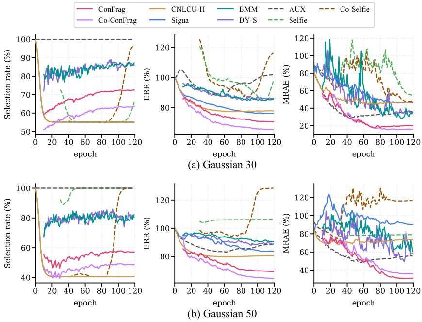
🔼 This figure compares the performance of ConFrag against five other strong baselines (CNLCU-H, BMM, DY-S, AUX, and Selfie) on the IMDB-Clean-B dataset. The comparison is made across three metrics: Selection rate, Error Residual Ratio (ERR), and Mean Relative Absolute Error (MRAE). The warm-up phase of training is excluded from the comparison. The figure shows ConFrag’s superior performance with the lowest ERR and MRAE while maintaining a reasonably high selection rate.
read the caption
Figure 5: Selection/ERR/MRAE comparison between ConFrag and strong baselines of CNLCU-H, BMM, DY-S, AUX and Selfie on IMDB-Clean-B. We exclude the performance during the warm-up.
🔼 The figure compares the performance of ConFrag against five strong baseline methods (CNLCU-H, BMM, DY-S, AUX, and Selfie) on the IMDB-Clean-B dataset with respect to selection rate, error residual ratio (ERR), and mean relative absolute error (MRAE). It visualizes these metrics over training epochs, excluding the initial warm-up phase. The graph demonstrates ConFrag’s superior performance in achieving a low ERR and MRAE while maintaining a competitive selection rate.
read the caption
Figure 5: Selection/ERR/MRAE comparison between ConFrag and strong baselines of CNLCU-H, BMM, DY-S, AUX and Selfie on IMDB-Clean-B. We exclude the performance during the warm-up.
More on tables
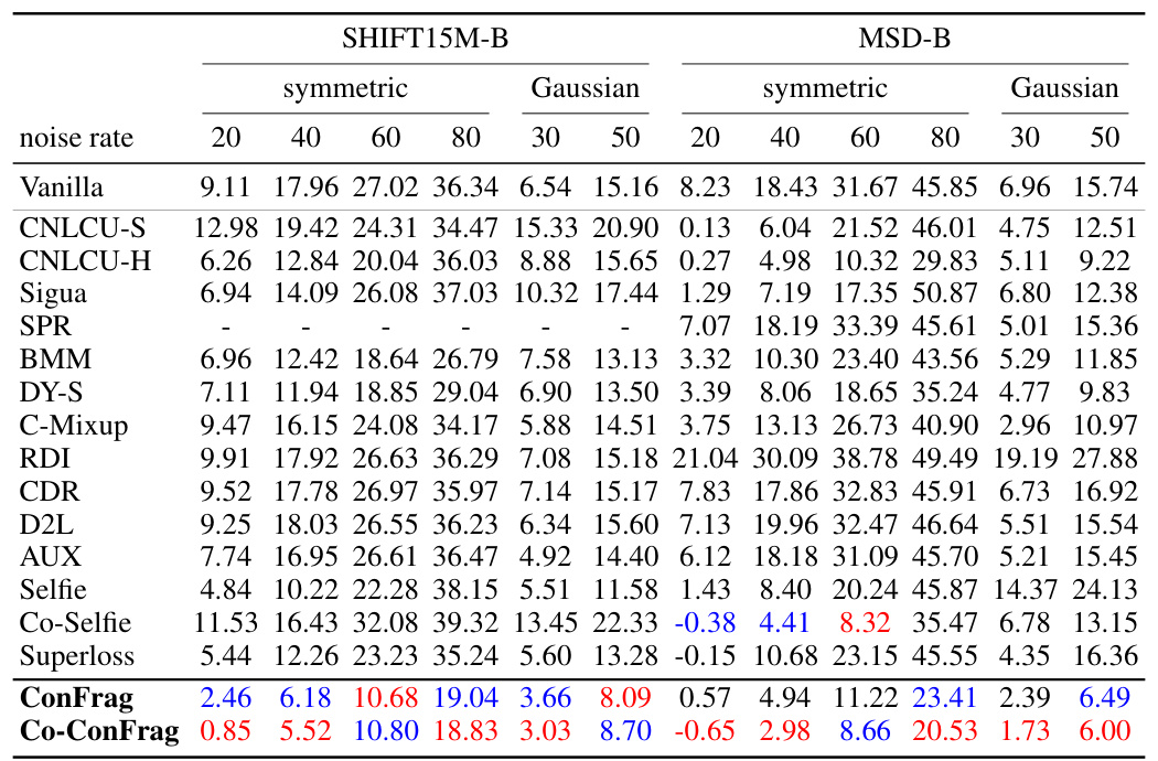
🔼 This table presents a comparison of the Mean Relative Absolute Error (MRAE) achieved by various methods (including ConFrag and fourteen baselines) on five different datasets with various types of noise. Lower MRAE values indicate better performance. A negative MRAE indicates the method outperforms the noise-free model. The results are averaged over three runs with different random seeds, and the best and second-best performing methods are highlighted.
read the caption
Table 1: Comparison of Mean Relative Absolute Error (%) over the noise-free trained model on the AFAD-B, IMDB-Clean-B, IMDB-WIKI-B, SHIFT15M-B, and MSD-B datasets. Lower is better. A negative value indicates it performs even better than the noise-free model. The results are the mean of three random seed experiments. The best and the second best methods are respectively marked in red and blue. CNLCU-S/H, Co-Selfie, and Co-ConFrag use dual networks to teach each other as done in Han et al. [2018]. SPR [Wang et al., 2022] fails to run for SHIFT15M-B due to excessive memory usage.

🔼 This table compares the performance of ConFrag and fourteen other state-of-the-art baselines on six benchmark datasets with varying types and amounts of noise. The Mean Relative Absolute Error (MRAE), a metric which accounts for noise severity, is used to measure performance, and lower values represent better performance. The table shows results for symmetric and Gaussian noise at different noise levels.
read the caption
Table 1: Comparison of Mean Relative Absolute Error (%) over the noise-free trained model on the AFAD-B, IMDB-Clean-B, IMDB-WIKI-B, SHIFT15M-B, and MSD-B datasets. Lower is better. A negative value indicates it performs even better than the noise-free model. The results are the mean of three random seed experiments. The best and the second best methods are respectively marked in red and blue. CNLCU-S/H, Co-Selfie, and Co-ConFrag use dual networks to teach each other as done in Han et al. [2018]. SPR [Wang et al., 2022] fails to run for SHIFT15M-B due to excessive memory usage.
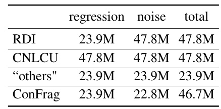
🔼 This table compares the number of parameters used in different methods for regression and noise mitigation. The ‘regression’ column indicates the number of parameters dedicated to the regression model itself. The ’noise’ column shows the number of parameters used specifically for handling noisy labels. The ‘others’ category groups several methods whose parameter counts are similar. Finally, ConFrag’s parameter counts are shown separately.
read the caption
Table 3: Parameter size comparison. regression: parameters for regression, noise: parameters to mitigate noisy labels, 'others': SPR, CDR, D2L, C-Mixup, Sigua, Selfie, BMM, DY-S, Superloss.

🔼 This table presents a comparison of the Mean Relative Absolute Error (MRAE) achieved by ConFrag and 14 other state-of-the-art baselines on five benchmark datasets. The MRAE is calculated relative to a noise-free model. Lower MRAE indicates better performance. The table includes results for different noise levels (symmetric and Gaussian) and dataset types (image-based age prediction, commodity price prediction, music production year estimation). The best and second-best performing methods are highlighted.
read the caption
Table 1: Comparison of Mean Relative Absolute Error (%) over the noise-free trained model on the AFAD-B, IMDB-Clean-B, IMDB-WIKI-B, SHIFT15M-B, and MSD-B datasets. Lower is better. A negative value indicates it performs even better than the noise-free model. The results are the mean of three random seed experiments. The best and the second best methods are respectively marked in red and blue. CNLCU-S/H, Co-Selfie, and Co-ConFrag use dual networks to teach each other as done in Han et al. [2018]. SPR [Wang et al., 2022] fails to run for SHIFT15M-B due to excessive memory usage.
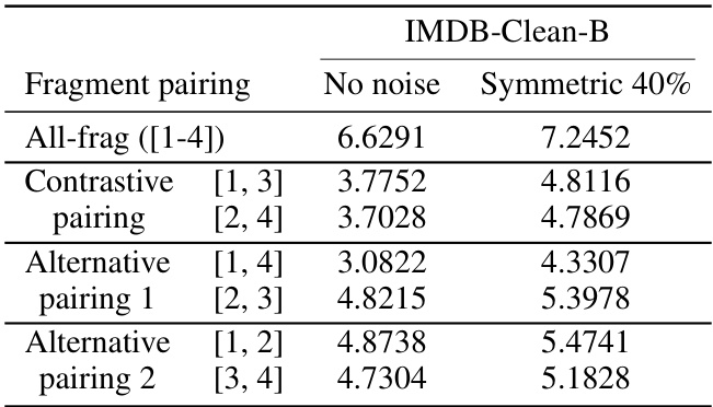
🔼 This table presents a comparison of the mean prediction depths achieved by different fragment pairing strategies in feature extractor learning tasks. It compares the performance of using all fragments, contrastive fragment pairings, and alternative fragment pairings when the number of fragments (F) is set to 4. The mean prediction depth is a metric that indicates how early in the network layers a sample’s class can be correctly predicted. Lower prediction depths generally indicate better generalization and less memorization. The table shows the mean prediction depths for both datasets with no noise and with symmetric 40% noise added.
read the caption
Table 5: Comparison of mean prediction depths of feature extractor learning tasks for all-frag, contrastive fragment pairing, and alternative fragmentation pairings when F = 4.

🔼 This table presents a comparison of the Mean Relative Absolute Error (MRAE) achieved by ConFrag and fourteen other state-of-the-art baselines on five benchmark datasets. The MRAE is calculated as the difference between the model’s Mean Absolute Error (MAE) with and without noise, normalized by the noise-free MAE. Lower MRAE values indicate better performance. The table showcases results for various noise levels (20%, 40%, 60%, 80% symmetric noise; 30%, 50% Gaussian noise) and highlights the best and second-best performing methods for each dataset and noise type. The use of dual networks in several methods is also noted.
read the caption
Table 1: Comparison of Mean Relative Absolute Error (%) over the noise-free trained model on the AFAD-B, IMDB-Clean-B, IMDB-WIKI-B, SHIFT15M-B, and MSD-B datasets. Lower is better. A negative value indicates it performs even better than the noise-free model. The results are the mean of three random seed experiments. The best and the second best methods are respectively marked in red and blue. CNLCU-S/H, Co-Selfie, and Co-ConFrag use dual networks to teach each other as done in Han et al. [2018]. SPR [Wang et al., 2022] fails to run for SHIFT15M-B due to excessive memory usage.

🔼 This table presents a comparison of the Mean Relative Absolute Error (MRAE) achieved by ConFrag and 14 other state-of-the-art baselines on five benchmark datasets. The MRAE is calculated relative to a noise-free model, with lower values indicating better performance. The results showcase ConFrag’s consistent superiority across different datasets and noise types (symmetric and Gaussian). The table also highlights the use of dual networks in some methods.
read the caption
Table 1: Comparison of Mean Relative Absolute Error (%) over the noise-free trained model on the AFAD-B, IMDB-Clean-B, IMDB-WIKI-B, SHIFT15M-B, and MSD-B datasets. Lower is better. A negative value indicates it performs even better than the noise-free model. The results are the mean of three random seed experiments. The best and the second best methods are respectively marked in red and blue. CNLCU-S/H, Co-Selfie, and Co-ConFrag use dual networks to teach each other as done in Han et al. [2018]. SPR [Wang et al., 2022] fails to run for SHIFT15M-B due to excessive memory usage.

🔼 This table presents a comparison of the Mean Relative Absolute Error (MRAE) achieved by ConFrag and fourteen baseline methods across five different datasets (AFAD-B, IMDB-Clean-B, IMDB-WIKI-B, SHIFT15M-B, and MSD-B) with varying levels of symmetric and Gaussian noise. Lower MRAE values indicate better performance. The table highlights the best and second-best performing methods for each noise level and dataset, demonstrating ConFrag’s superior performance, even outperforming the noise-free model in some cases. The note clarifies that Co-ConFrag and related methods use a dual-network training approach, and SPR failed to run on one dataset due to memory constraints.
read the caption
Table 1: Comparison of Mean Relative Absolute Error (%) over the noise-free trained model on the AFAD-B, IMDB-Clean-B, IMDB-WIKI-B, SHIFT15M-B, and MSD-B datasets. Lower is better. A negative value indicates it performs even better than the noise-free model. The results are the mean of three random seed experiments. The best and the second best methods are respectively marked in red and blue. CNLCU-S/H, Co-Selfie, and Co-ConFrag use dual networks to teach each other as done in Han et al. [2018]. SPR [Wang et al., 2022] fails to run for SHIFT15M-B due to excessive memory usage.
🔼 This table presents a comparison of the Mean Relative Absolute Error (MRAE) achieved by ConFrag and fourteen other state-of-the-art baselines on five different benchmark datasets. The datasets cover diverse domains and types of noise (symmetric and Gaussian). Lower MRAE values indicate better performance. The table highlights ConFrag’s robustness and superior performance compared to other methods.
read the caption
Table 1: Comparison of Mean Relative Absolute Error (%) over the noise-free trained model on the AFAD-B, IMDB-Clean-B, IMDB-WIKI-B, SHIFT15M-B, and MSD-B datasets. Lower is better. A negative value indicates it performs even better than the noise-free model. The results are the mean of three random seed experiments. The best and the second best methods are respectively marked in red and blue. CNLCU-S/H, Co-Selfie, and Co-ConFrag use dual networks to teach each other as done in Han et al. [2018]. SPR [Wang et al., 2022] fails to run for SHIFT15M-B due to excessive memory usage.

🔼 This table presents a comparison of the Mean Relative Absolute Error (MRAE) achieved by ConFrag and fourteen other state-of-the-art baselines on five different datasets. The MRAE is calculated as the difference between the model’s MAE on noisy data and the MAE on clean data, expressed as a percentage. Lower MRAE values indicate better performance. The table shows results for different types of noise (symmetric and Gaussian) and varying noise rates. The best performing models are highlighted in red and blue.
read the caption
Table 1: Comparison of Mean Relative Absolute Error (%) over the noise-free trained model on the AFAD-B, IMDB-Clean-B, IMDB-WIKI-B, SHIFT15M-B, and MSD-B datasets. Lower is better. A negative value indicates it performs even better than the noise-free model. The results are the mean of three random seed experiments. The best and the second best methods are respectively marked in red and blue. CNLCU-S/H, Co-Selfie, and Co-ConFrag use dual networks to teach each other as done in Han et al. [2018]. SPR [Wang et al., 2022] fails to run for SHIFT15M-B due to excessive memory usage.
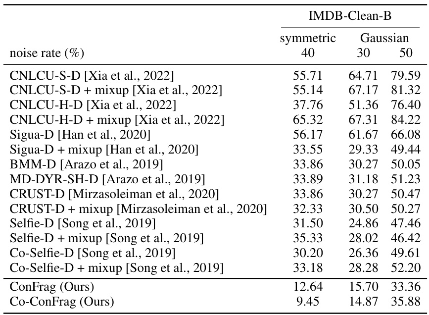
🔼 This table presents a comparison of the Mean Relative Absolute Error (MRAE) achieved by ConFrag and fourteen other state-of-the-art baselines on five different datasets. The MRAE is calculated relative to a noise-free model, allowing for negative values indicating superior performance. Results are averaged across three random trials. The datasets cover diverse domains and are designed to evaluate performance under varying degrees of symmetric and Gaussian noise.
read the caption
Table 1: Comparison of Mean Relative Absolute Error (%) over the noise-free trained model on the AFAD-B, IMDB-Clean-B, IMDB-WIKI-B, SHIFT15M-B, and MSD-B datasets. Lower is better. A negative value indicates it performs even better than the noise-free model. The results are the mean of three random seed experiments. The best and the second best methods are respectively marked in red and blue. CNLCU-S/H, Co-Selfie, and Co-ConFrag use dual networks to teach each other as done in Han et al. [2018]. SPR [Wang et al., 2022] fails to run for SHIFT15M-B due to excessive memory usage.

🔼 This table presents a comparison of the Mean Relative Absolute Error (MRAE) achieved by ConFrag and fourteen baseline methods across five datasets with varying levels of symmetric and Gaussian noise. Lower MRAE values indicate better performance. The table highlights ConFrag’s superior performance in most scenarios and showcases its robustness against different types of noise.
read the caption
Table 1: Comparison of Mean Relative Absolute Error (%) over the noise-free trained model on the AFAD-B, IMDB-Clean-B, IMDB-WIKI-B, SHIFT15M-B, and MSD-B datasets. Lower is better. A negative value indicates it performs even better than the noise-free model. The results are the mean of three random seed experiments. The best and the second best methods are respectively marked in red and blue. CNLCU-S/H, Co-Selfie, and Co-ConFrag use dual networks to teach each other as done in Han et al. [2018]. SPR [Wang et al., 2022] fails to run for SHIFT15M-B due to excessive memory usage.

🔼 This table presents a comparison of the Mean Relative Absolute Error (MRAE) achieved by ConFrag and fourteen other state-of-the-art baselines across five different datasets (AFAD-B, IMDB-Clean-B, IMDB-WIKI-B, SHIFT15M-B, and MSD-B). For each dataset, results are shown for both symmetric and Gaussian noise at different noise levels (20%, 40%, 60%, 80% for symmetric, 30%, 50% for Gaussian). Lower MRAE values indicate better performance. The table highlights the best and second-best performing methods in red and blue, respectively, and notes that the SPR method failed to execute on one of the datasets due to memory constraints.
read the caption
Table 1: Comparison of Mean Relative Absolute Error (%) over the noise-free trained model on the AFAD-B, IMDB-Clean-B, IMDB-WIKI-B, SHIFT15M-B, and MSD-B datasets. Lower is better. A negative value indicates it performs even better than the noise-free model. The results are the mean of three random seed experiments. The best and the second best methods are respectively marked in red and blue. CNLCU-S/H, Co-Selfie, and Co-ConFrag use dual networks to teach each other as done in Han et al. [2018]. SPR [Wang et al., 2022] fails to run for SHIFT15M-B due to excessive memory usage.
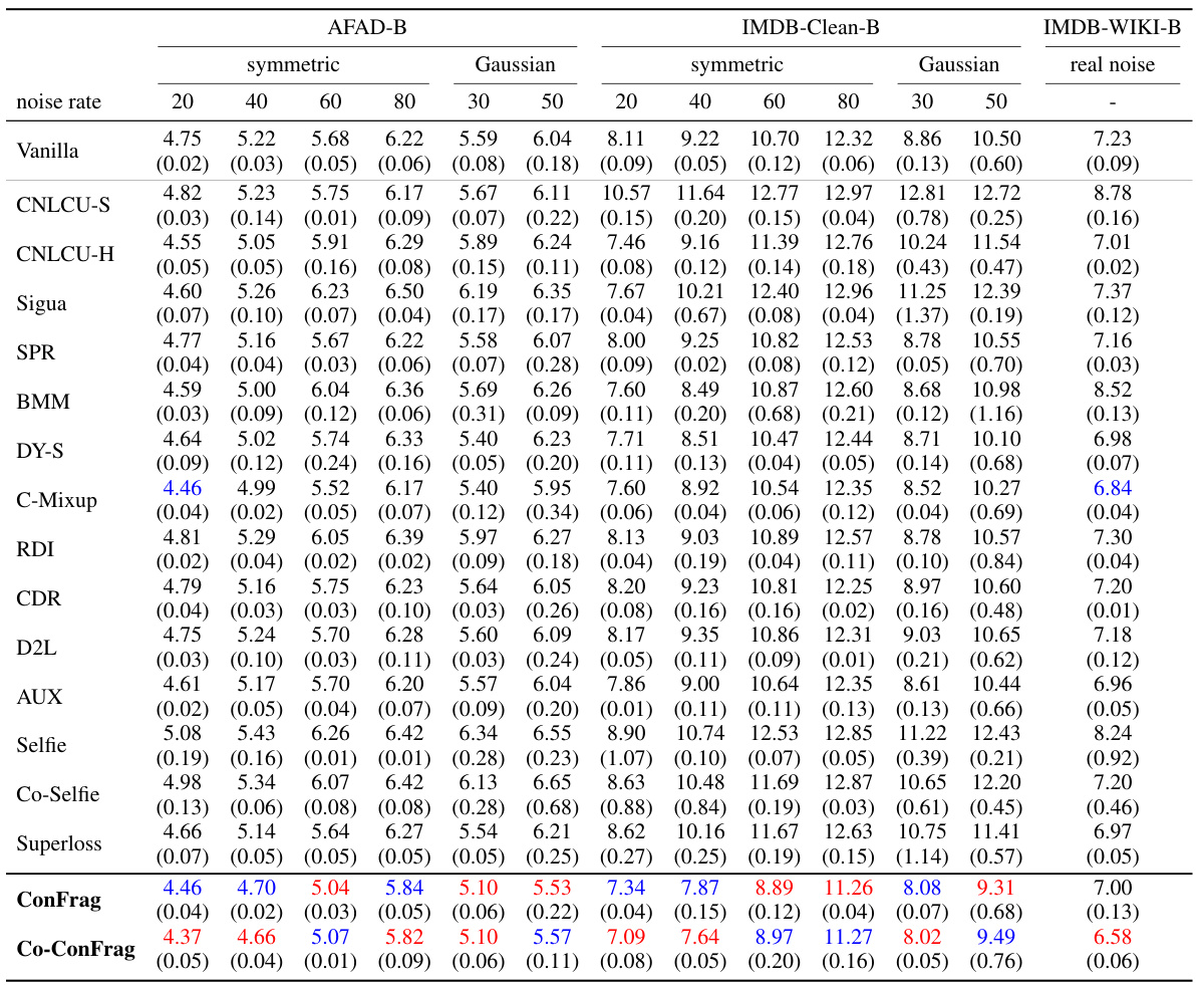
🔼 This table presents a comparison of the Mean Relative Absolute Error (MRAE) achieved by various methods (including ConFrag) on five different datasets with varying noise levels (symmetric and Gaussian noise). Lower MRAE values indicate better performance. The table highlights the best-performing methods in each scenario and notes that Co-ConFrag uses a dual-network training strategy. The inability of SPR to run on one dataset is also noted.
read the caption
Table 1: Comparison of Mean Relative Absolute Error (%) over the noise-free trained model on the AFAD-B, IMDB-Clean-B, IMDB-WIKI-B, SHIFT15M-B, and MSD-B datasets. Lower is better. A negative value indicates it performs even better than the noise-free model. The results are the mean of three random seed experiments. The best and the second best methods are respectively marked in red and blue. CNLCU-S/H, Co-Selfie, and Co-ConFrag use dual networks to teach each other as done in Han et al. [2018]. SPR [Wang et al., 2022] fails to run for SHIFT15M-B due to excessive memory usage.
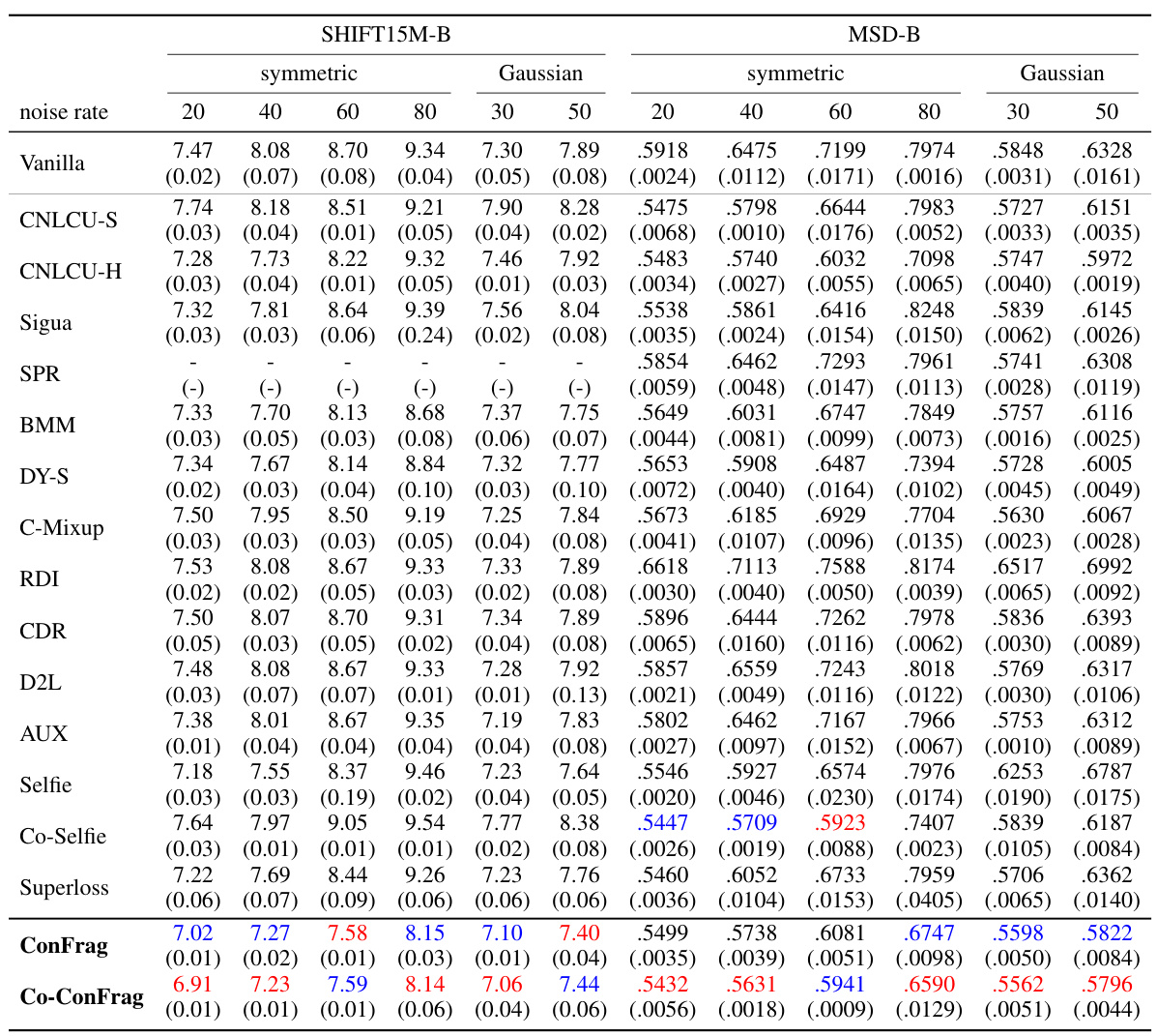
🔼 This table presents a comparison of the Mean Relative Absolute Error (MRAE) achieved by ConFrag and fourteen baseline methods across five different datasets (AFAD-B, IMDB-Clean-B, IMDB-WIKI-B, SHIFT15M-B, and MSD-B). The MRAE is calculated relative to a noise-free model. Results are shown for various levels of symmetric and Gaussian noise, highlighting ConFrag’s robustness and superior performance compared to other state-of-the-art methods. A negative MRAE indicates that the model outperforms the noise-free model.
read the caption
Table 1: Comparison of Mean Relative Absolute Error (%) over the noise-free trained model on the AFAD-B, IMDB-Clean-B, IMDB-WIKI-B, SHIFT15M-B, and MSD-B datasets. Lower is better. A negative value indicates it performs even better than the noise-free model. The results are the mean of three random seed experiments. The best and the second best methods are respectively marked in red and blue. CNLCU-S/H, Co-Selfie, and Co-ConFrag use dual networks to teach each other as done in Han et al. [2018]. SPR [Wang et al., 2022] fails to run for SHIFT15M-B due to excessive memory usage.
Full paper#
