TL;DR#
Topological data analysis (TDA) offers topological loss functions for optimizing object shapes to exhibit desired topological properties. However, using gradient descent for optimization is slow due to extremely sparse gradients, affecting only a few coordinates. This sparsity also hinders applications to large datasets and black-box autoencoders where gradients are unavailable.
This paper proposes using diffeomorphic interpolation to address this challenge. The method smoothly interpolates sparse gradients, creating a dense vector field applicable to the entire dataset. This improved efficiency allows for optimization of much larger datasets and facilitates the application of topological priors to black-box autoencoders, enabling faster convergence and better interpretability of latent spaces. This significantly advances the field of topological optimization, making it feasible for much larger datasets and complex machine learning applications.
Key Takeaways#
Why does it matter?#
This paper is important because it offers a novel solution to a significant challenge in topological optimization: the sparsity of gradients. By introducing diffeomorphic interpolation, it enables efficient optimization of point clouds at unprecedented scales and facilitates the application of topological priors to black-box autoencoders. This opens new avenues for research in various fields such as shape analysis, machine learning, and topological data analysis.
Visual Insights#

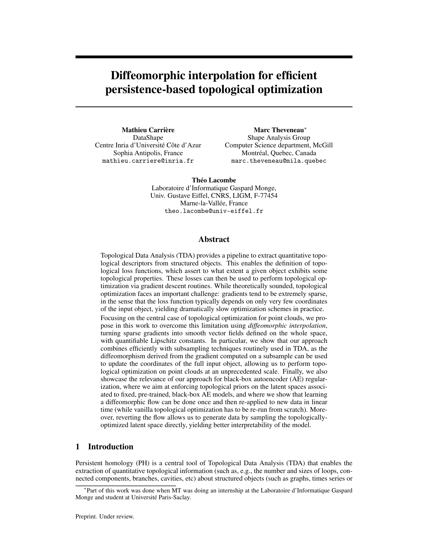
🔼 This figure illustrates the Vietoris-Rips filtration process on a point cloud. It shows how, as a parameter ’t’ increases, circles of increasing radii are formed around each point. Simplices (lines, triangles, etc.) are added to a simplicial complex whenever the points are within a distance ’t’ of each other. The evolution of topological features (loops in this case) as ’t’ changes is shown in the sequence of diagrams. Finally, a persistence diagram summarizes the birth and death times of these topological features, providing quantitative topological information.
read the caption
Figure 1: Illustration of the Vietoris-Rips filtration on a point cloud in Rd, focusing on one-dimensional topological features (loops). When the filtration parameter t increases, loops appear and disappear in the filtration. These values are accounted in the resulting persistence diagram (right).

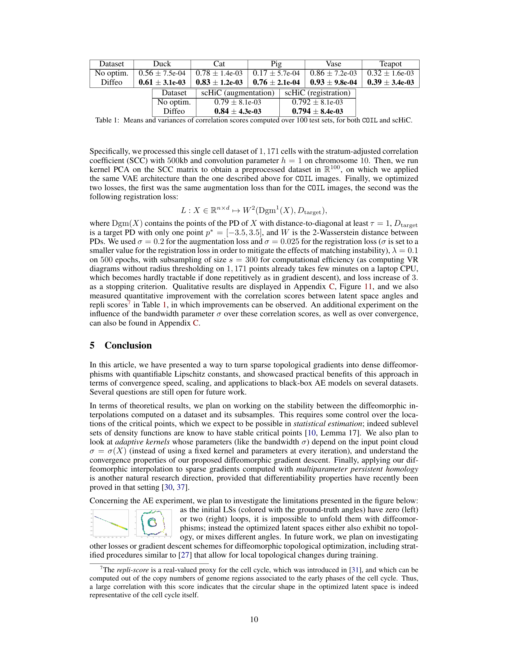
🔼 This table presents the mean and variance of Pearson correlation scores calculated across 100 test sets for the COIL and scHiC datasets. The scores measure the correlation between ground-truth angles and angles computed from topologically optimized latent spaces. The table compares these scores for experiments with and without diffeomorphic interpolation, demonstrating the improvement in correlation achieved using diffeomorphic interpolation.
read the caption
Table 1: Means and variances of correlation scores computed over 100 test sets, for both COIL and scHiC.
In-depth insights#
Diffeomorphic TDA#
Diffeomorphic TDA represents a novel approach to address the challenges of traditional topological data analysis (TDA) in topological optimization. Standard TDA methods often produce sparse gradients, leading to slow and inefficient optimization. Diffeomorphic interpolation overcomes this by transforming sparse gradients into smooth vector fields defined across the entire space. This ensures that gradient descent updates affect more data points, speeding up the optimization process considerably. The method’s effectiveness is further enhanced by its compatibility with subsampling techniques, allowing the application of TDA to significantly larger datasets than previously possible. Quantifiable Lipschitz constants provide a measure of smoothness and stability, adding to the theoretical rigor of the approach. The successful application of diffeomorphic TDA to black-box autoencoder regularization demonstrates its versatility and potential for broader impact in machine learning. The ability to generate data by sampling the topologically optimized latent space offers improved model interpretability and allows for creative data augmentation.
Gradient Interpolation#
The concept of ‘Gradient Interpolation’ in topological data analysis addresses a critical challenge: sparse gradients produced by traditional topological loss functions. These sparse gradients hinder efficient optimization, as only a small subset of data points is updated at each iteration. Interpolation techniques create a smooth, dense vector field from the sparse gradient, enabling all data points to be considered during optimization. This leads to faster convergence and improved efficiency, particularly beneficial when dealing with large datasets. Diffeomorphic interpolation, a specific approach, guarantees that the interpolation maintains important properties like smoothness and invertibility. This is crucial as it ensures the optimization process continues to effectively decrease the loss function while preserving the topological properties of interest. The ability to smoothly interpolate gradients opens up new possibilities for applying topological optimization to larger, more complex problems and diverse applications such as regularizing black-box autoencoders.
Subsampling TDA#
Subsampling techniques are crucial for scaling Topological Data Analysis (TDA) to massive datasets. Computational cost of TDA algorithms often scales poorly with data size, making analysis of large point clouds or complex networks intractable. Subsampling addresses this by analyzing a smaller, randomly selected subset of the data. This significantly reduces computation time, allowing for the processing of datasets previously deemed too large for TDA. The effectiveness of subsampling hinges on the stability of topological features, meaning that similar topological summaries should result from analyzing the subset and the full dataset. While subsampling introduces approximation errors, the inherent robustness of persistent homology often mitigates these errors, particularly when focusing on prominent topological features. However, careful consideration of subsampling strategies is needed to balance computational efficiency with the preservation of meaningful topological information. Strategies such as carefully choosing the subsample size and employing multiple subsamples can significantly impact the results. The interplay between subsampling and the choice of distance metric and topological features is a critical research area within TDA. Combining subsampling with efficient algorithms and advanced computational techniques can unlock the potential of TDA for truly large-scale data analysis. Subsampling remains a valuable tool for making TDA accessible and practical for a broader range of applications.
Autoencoder Regularization#
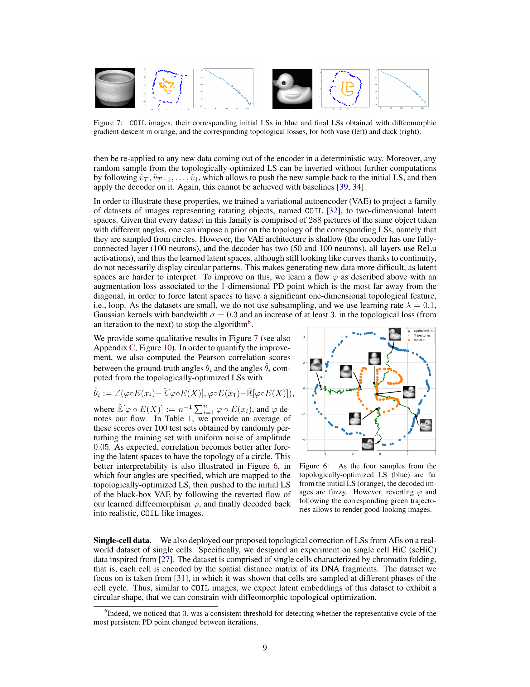
Autoencoder regularization, in the context of topological data analysis (TDA), offers a powerful technique to enforce topological priors on the latent space representations learned by autoencoders. By integrating topological loss functions into the autoencoder’s training objective, one can guide the learning process to produce latent spaces exhibiting desired topological structures. This is particularly valuable when dealing with complex data where preserving the underlying topology is crucial for downstream tasks. The method addresses the challenge of sparse gradients typically encountered in TDA-based optimization by employing diffeomorphic interpolation, enabling efficient optimization even at scale. Diffeomorphic flows ensure smooth transitions in the latent space, leading to improved stability and interpretability of the learned representations. The ability to learn a diffeomorphic map once and apply it efficiently to new data points is a key advantage. This technique can have significant implications for various applications, particularly where understanding and controlling the topological properties of latent representations is paramount. It allows for data generation by sampling from the optimized latent space and reversing the learned flow, resulting in enhanced data interpretability and model explainability.
Future Research#
Future research directions stemming from this work on diffeomorphic interpolation for topological optimization are multifaceted. Theoretical investigations should focus on rigorously establishing the stability of diffeomorphic interpolations under subsampling, potentially leveraging results on the stability of critical points in density functions. Algorithmic improvements could explore adaptive kernel functions where bandwidth is data-dependent, potentially improving efficiency and robustness. The impact of different kernel choices on convergence should also be thoroughly investigated. Applications warrant exploration beyond the current examples, considering diverse domains like graph analysis and time series data. Moreover, integration with other TDA methods like mapper and Ripser could enhance scalability and provide richer topological insights. Finally, a deeper examination of the relationship between the Lipschitz constant of the diffeomorphism and the convergence speed of the optimization process could lead to novel optimization strategies.
More visual insights#
More on figures
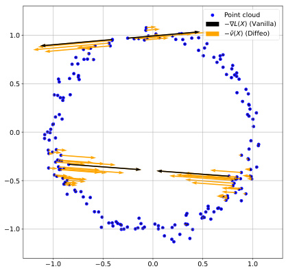
🔼 This figure illustrates the effect of diffeomorphic interpolation on a point cloud. The black arrows show the sparse gradient of a topological loss function, which only affects a few points. The orange arrows, generated by the diffeomorphic interpolation technique, show a smoother vector field extending the gradient to all points, enabling a more efficient optimization.
read the caption
Figure 2: (blue) A point cloud X, and (black) the negative gradient -∇L(X) of a simplification loss which aims at destroying the loop by collapsing the circle (reduce the loop's death time) and tearing it (increase the birth time). While ∇L(X) only affects four points in X, the diffeomorphic interpolation ῦ(X) (orange, σ = 0.1) is defined on Rd, hence extends smoothly to other points in X.

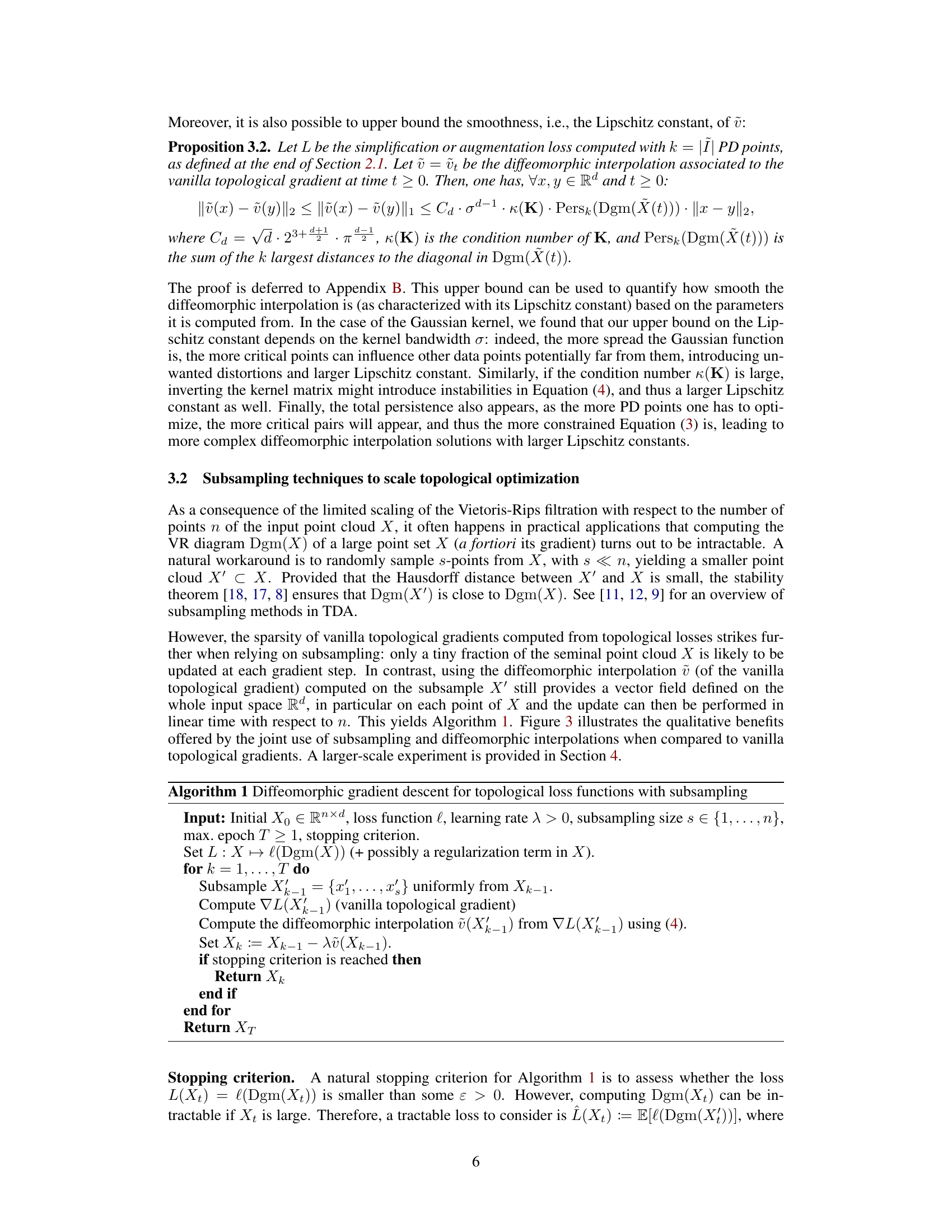
🔼 This figure showcases the benefits of combining subsampling with diffeomorphic interpolation for topological optimization. It compares the vanilla gradient descent approach (sparse updates) with the proposed approach (dense updates) using a topological simplification loss. The figure illustrates how diffeomorphic interpolation significantly improves the efficiency of the optimization process.
read the caption
Figure 3: Showcase of the usefulness of subsampling combined with diffeomorphic interpolations to minimize a topological simplification loss, with parameters λ = 0.1, s = 50, n = 500. (a) Initial point cloud X (blue), subsample X' (red), vanilla topological gradient on the subsample (black) and corresponding diffeomorphic interpolation (orange). (b) and (c), the point cloud Xt after running t = 100 and t = 500 steps of vanilla gradient descent. (d) the point cloud Xt after running t = 100 steps of diffeomorphic gradient descent.
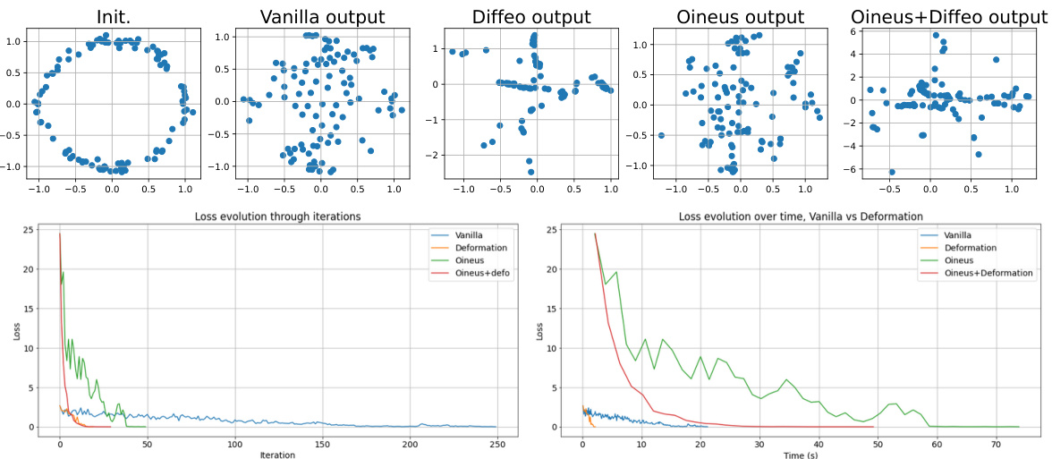
🔼 This figure compares four different methods for topological optimization: vanilla gradient descent, diffeomorphic interpolation, Oineus, and a combination of Oineus and diffeomorphic interpolation. The top row shows the initial and final point clouds for each method, illustrating the different ways they modify the point cloud to reduce the topological loss. The bottom row shows plots of the loss over iterations and over time for each method. The results demonstrate that the diffeomorphic interpolation and Oineus methods significantly outperform the vanilla gradient descent method in terms of loss reduction, and that combining Oineus with diffeomorphic interpolation yields the fastest convergence.
read the caption
Figure 4: (Top) From left to right: initial point cloud, and final point cloud for the different flows. (Bottom) Evolution of the losses with respect to the number of iterations and with respect to running time.

🔼 This figure compares the vanilla topological gradient descent and the diffeomorphic gradient descent methods on the Stanford Bunny dataset for topological augmentation. The left side shows the initial bunny point cloud and the results after different numbers of epochs (iterations) for both methods. The right side shows the loss evolution over the iterations. The vanilla gradient descent shows minimal changes even after 1000 epochs, while the diffeomorphic gradient descent achieves significant changes in a much shorter timeframe.
read the caption
Figure 5: From left to right: initial Stanford bunny X0, the point cloud after 1, 000 epochs of vanilla topological gradient descent (barely any changes), the point cloud after 200 epochs of diffeomorphic gradient descent, after 1,000 epochs, and eventually the evolution of losses for both methods over iterations.

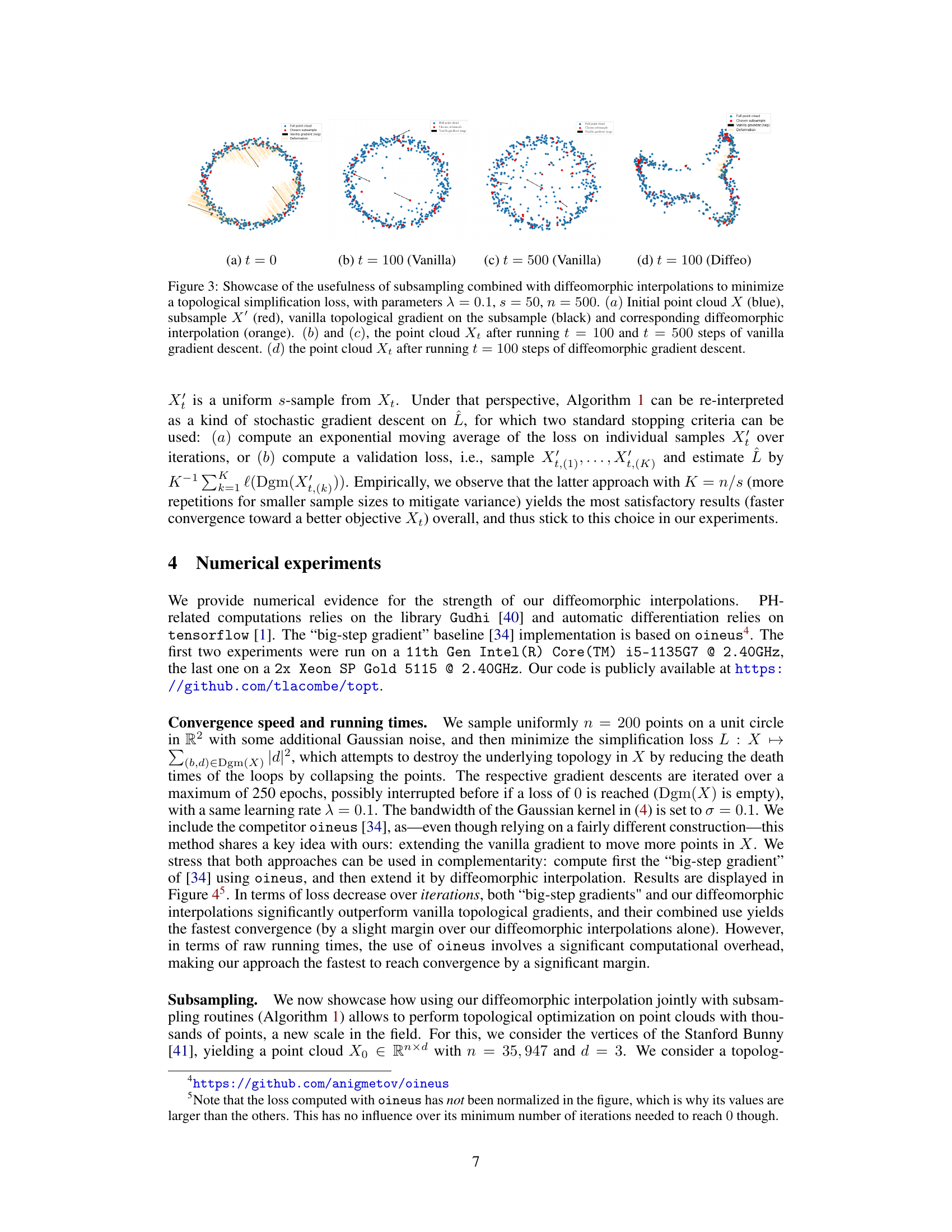
🔼 This figure shows the results of applying the proposed diffeomorphic interpolation method to the latent spaces of a variational autoencoder trained on COIL images (rotating objects). The left side shows the initial latent space (LS) for the vase image in blue, and how it transforms after gradient descent using the diffeomorphic approach in orange. The corresponding topological loss reduction is also plotted in a graph. The right side shows the same process but for the duck image. The method aims to improve the topological properties of the latent space by making it more circular, reflecting the circular motion of the objects.
read the caption
Figure 7: COIL images, their corresponding initial LSs in blue and final LSs obtained with diffeomorphic gradient descent in orange, and the corresponding topological losses, for both vase (left) and duck (right).

🔼 This figure shows the results of applying diffeomorphic interpolation to the latent spaces (LSs) of a variational autoencoder (VAE) trained on the COIL dataset. The initial LSs (blue) are compared to the final LSs (orange) obtained after applying the diffeomorphic gradient descent. The images show how the algorithm modifies the latent space to improve its topological properties, aiming for a circular structure, as indicated by the topological loss values shown for both the vase and duck objects.
read the caption
Figure 7: COIL images, their corresponding initial LSs in blue and final LSs obtained with diffeomorphic gradient descent in orange, and the corresponding topological losses, for both vase (left) and duck (right).

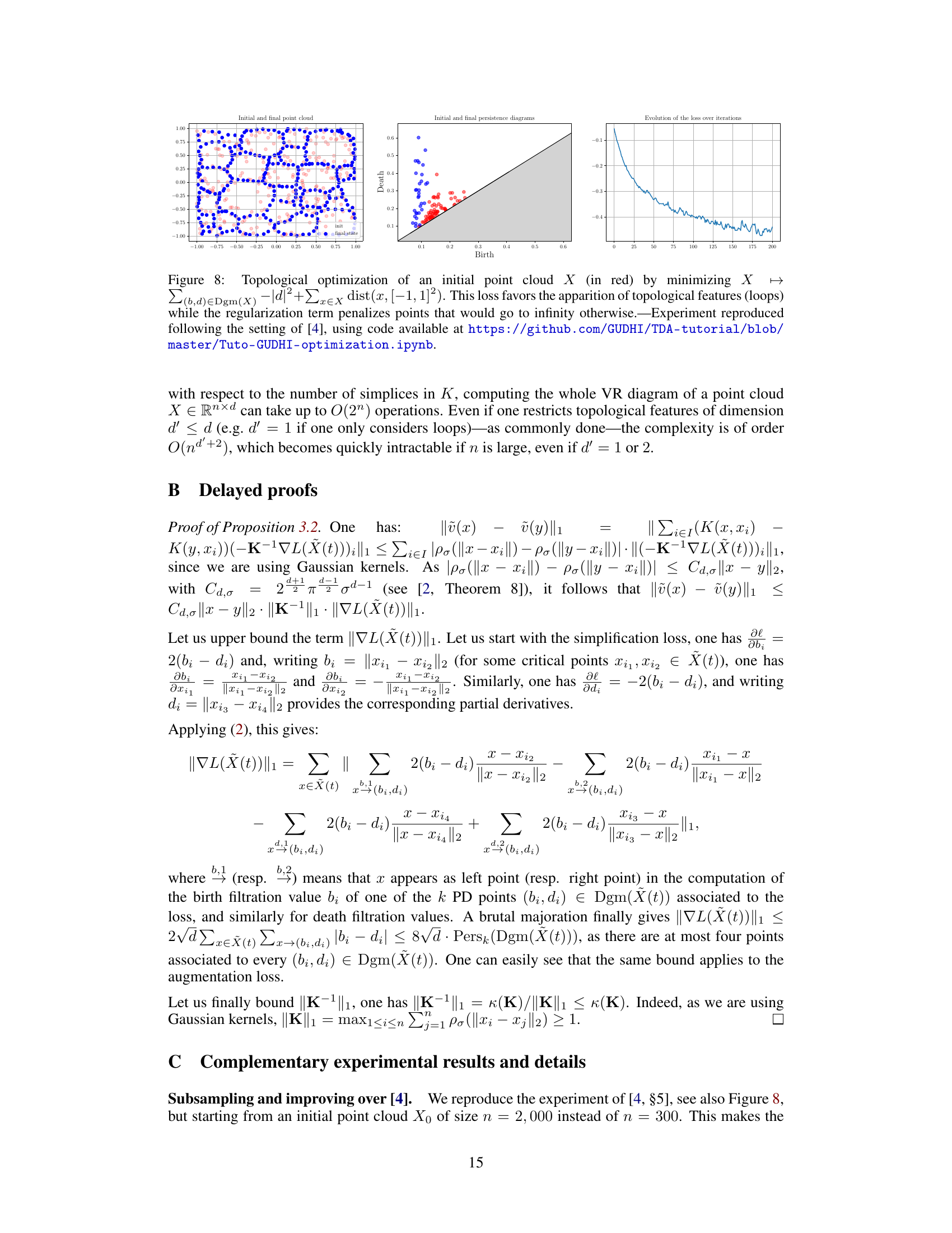
🔼 This figure shows the result of topological optimization on an initial point cloud. The objective function used encourages the formation of loops (1-dimensional topological features) while regularizing to prevent points from moving to infinity. The three subplots show (1) the initial and final point cloud, (2) the initial and final persistence diagrams, and (3) the loss function’s evolution over iterations. This experiment was replicated from a previously published work, with code provided for reproducibility.
read the caption
Figure 8: Topological optimization of an initial point cloud X (in red) by minimizing X → Σ(b,d)∈Dgm(X) |d|² + x∈X dist(x, [−1, 1]²). This loss favors the apparition of topological features (loops) while the regularization term penalizes points that would go to infinity otherwise. Experiment reproduced following the setting of [4], using code available at https://github.com/GUDHI/TDA-tutorial/blob/master/Tuto-GUDHI-optimization.ipynb.

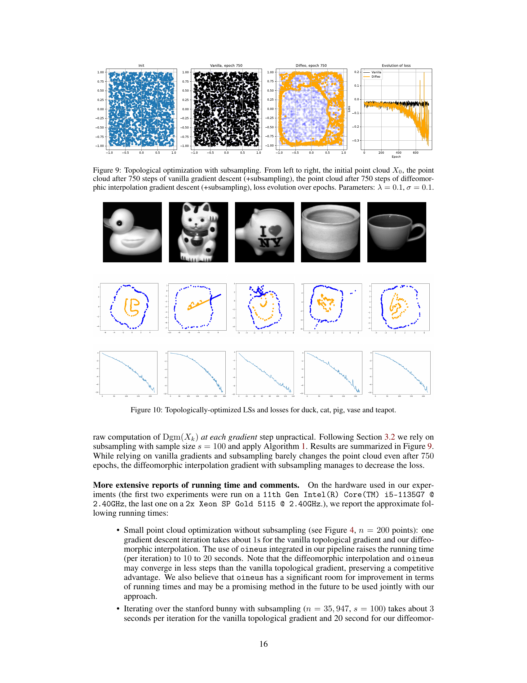
🔼 This figure shows the results of topological optimization using both vanilla gradient descent and the proposed diffeomorphic interpolation method, with subsampling applied to handle large datasets. The left three panels display the initial point cloud and the results after 750 epochs of vanilla gradient descent and diffeomorphic interpolation, respectively. The rightmost panel shows the evolution of the loss function over the 750 epochs, clearly demonstrating the faster convergence and lower final loss achieved by the diffeomorphic interpolation method. Subsampling is a crucial element, allowing the algorithm to scale to larger datasets.
read the caption
Figure 9: Topological optimization with subsampling. From left to right, the initial point cloud X0, the point cloud after 750 steps of vanilla gradient descent (+subsampling), the point cloud after 750 steps of diffeomorphic interpolation gradient descent (+subsampling), loss evolution over epochs. Parameters: λ = 0.1, σ = 0.1.

🔼 This figure shows the results of applying the proposed diffeomorphic interpolation method to latent spaces (LSs) of a variational autoencoder (VAE) trained on the COIL dataset. The top row displays the original images of five different objects (duck, cat, pig, vase, and teapot). The middle row shows the latent spaces obtained after applying the proposed method (orange dots) and the original latent spaces (blue dots). The bottom row shows the evolution of the topological loss during the optimization process for each object. The results demonstrate that the proposed method effectively improves the topological properties of the latent spaces.
read the caption
Figure 10: Topologically-optimized LSs and losses for duck, cat, pig, vase and teapot.

🔼 The figure shows the result of applying different gradient descent methods to minimize a topological loss function. The top row displays the initial point cloud and the final point cloud obtained after applying vanilla gradient descent, diffeomorphic interpolation, Oineus algorithm, and a combination of Oineus and diffeomorphic interpolation. The bottom row shows the evolution of the loss function with respect to the number of iterations and the running time for each method. The results demonstrate that the diffeomorphic interpolation and Oineus methods converge faster and achieve lower loss values compared to vanilla gradient descent, and the combination of Oineus and diffeomorphic interpolation shows the best performance. The visualizations help to compare different gradient descent approaches for topological optimization and assess their effectiveness.
read the caption
Figure 4: (Top) From left to right: initial point cloud, and final point cloud for the different flows. (Bottom) Evolution of the losses with respect to the number of iterations and with respect to running time.

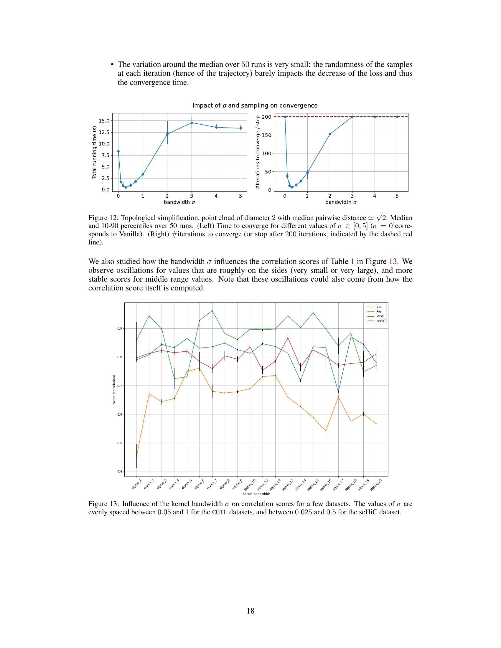
🔼 This figure shows the impact of the bandwidth (σ) parameter on the convergence speed of the diffeomorphic interpolation method proposed in the paper. The left panel displays the total running time to converge (or reach the maximum iteration limit of 200), while the right panel displays the number of iterations required for convergence. Both panels show median values and 10th and 90th percentiles from 50 runs of the algorithm. The results demonstrate that a value of σ around 0.3 provides a good balance between convergence speed and the number of iterations, while extremely small or large values of σ hinder convergence.
read the caption
Figure 12: Topological simplification, point cloud of diameter 2 with median pairwise distance ~ √2. Median and 10–90 percentiles over 50 runs. (Left) Time to converge for different values of σ∈ [0,5] (σ = 0 corresponds to Vanilla). (Right) #iterations to converge (or stop after 200 iterations, indicated by the dashed red line).
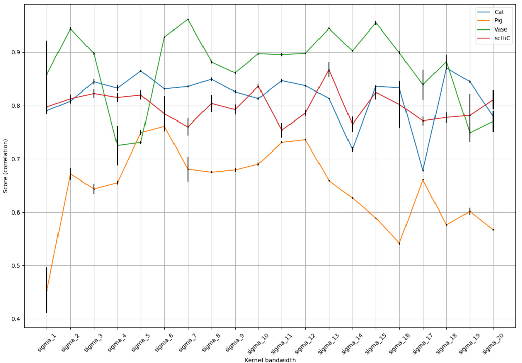
🔼 This figure shows how the correlation scores between latent space angles and repli scores vary with different kernel bandwidths (σ) for several datasets (Cat, Pig, Vase, and scHiC). The x-axis represents the kernel bandwidth, and the y-axis shows the correlation scores. The plot reveals oscillations in the correlation scores for very small or large bandwidths, suggesting more stable scores in the middle range. These oscillations might also stem from how the correlation scores are calculated.
read the caption
Figure 13: Influence of the kernel bandwidth σ on correlation scores for a few datasets. The values of σ are evenly spaced between 0.05 and 1 for the COIL datasets, and between 0.025 and 0.5 for the scHiC dataset.
Full paper#
