TL;DR#
Classical bias-variance theory posits a U-shaped relationship between model complexity and generalization error. However, recent research reveals the phenomenon of “double descent,” where generalization error initially increases, then decreases again with increasing model complexity. Existing explanations primarily focus on the over-parameterized regime. This research paper investigates the under-parameterized regime.
This work presents two novel examples exhibiting double descent in the under-parameterized regime. These findings challenge existing theories, suggesting that the relationship between data points, parameters, and generalization is more complex than previously understood. The study focuses on how the spectral properties of the sample covariance matrix, particularly eigenvector alignment and spectrum, influence the location and occurrence of the double descent peak.
Key Takeaways#
Why does it matter?#
This paper challenges the conventional understanding of the bias-variance trade-off in regression by demonstrating under-parameterized double descent in simple linear models. This finding has significant implications for model selection and regularization, particularly in scenarios with limited data. The research opens up new avenues for investigating similar phenomena in more complex models and architectures, advancing the field of machine learning.
Visual Insights#

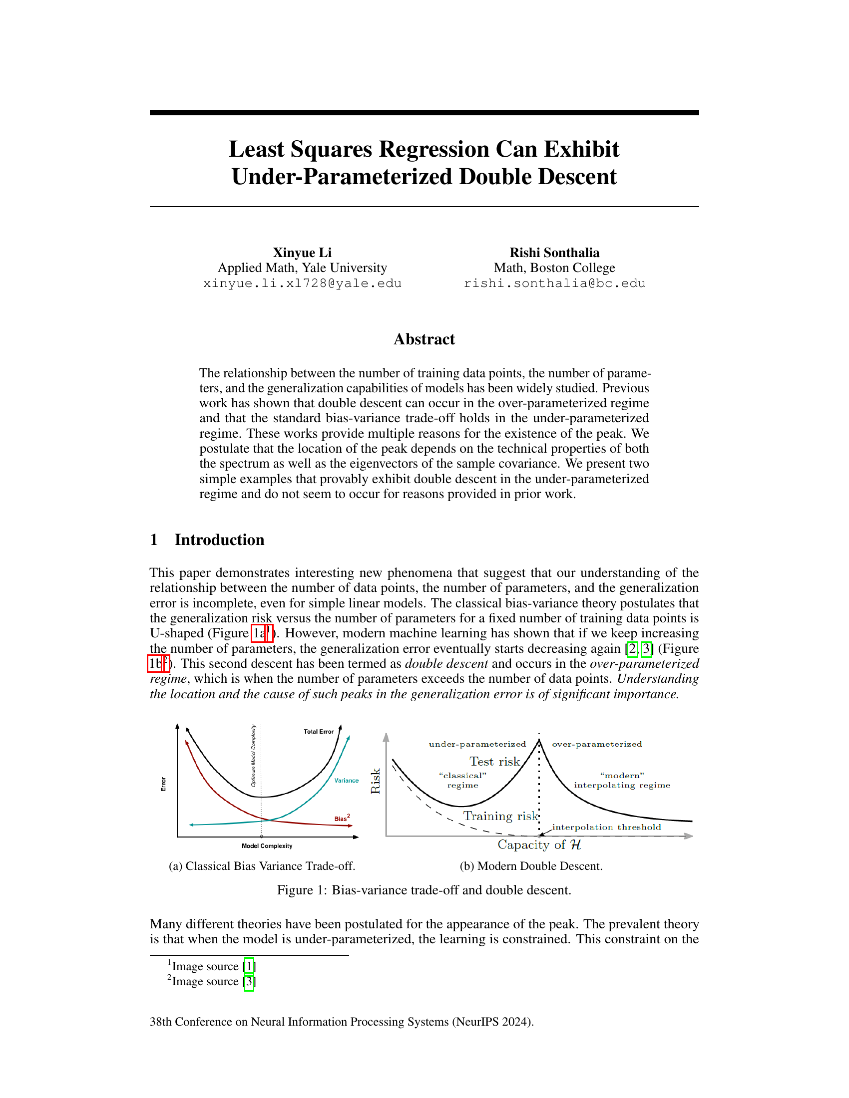
🔼 This figure shows two plots illustrating the concepts of bias-variance trade-off and double descent in machine learning. (a) Classical Bias Variance Trade-off: This plot displays the classical relationship between model complexity and total error, which is composed of bias and variance. It shows that as model complexity increases, bias decreases while variance increases, leading to a U-shaped curve representing total error. (b) Modern Double Descent: This plot demonstrates the phenomenon of double descent. It shows that when model complexity increases beyond the number of data points (i.e., the interpolation threshold), generalization error first increases before decreasing again. This behavior suggests a more nuanced relationship between model capacity and generalization performance.
read the caption
Figure 1: Bias-variance trade-off and double descent.
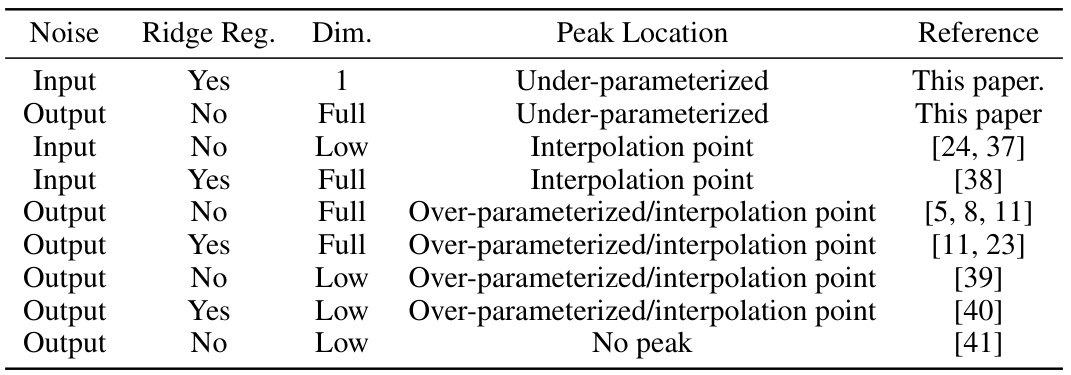
🔼 This table summarizes the findings of various studies on double descent in linear regression and denoising, comparing different assumptions regarding noise, ridge regularization, and data dimensionality. It shows the location of the double descent peak (under-parameterized, over-parameterized, or interpolation point) observed in each study, along with references. A notable addition is the inclusion of the current paper’s findings for under-parameterized double descent.
read the caption
Table 1: Table showing various assumptions on the data and the location of the double descent peak for linear regression and denoising. We only present a subset of references for each problem setting. For the low rank setting in this paper, see Appendix F.
In-depth insights#
Underparameterized Peaks#
The concept of “Underparameterized Peaks” in regression analysis challenges the traditional bias-variance tradeoff. It suggests that the generalization error, instead of monotonically decreasing with model complexity in the underparameterized regime, can exhibit a peak before eventually decreasing. This phenomenon contradicts the established understanding that simpler models are inherently less prone to overfitting. The location of this peak is crucial, often linked to the alignment between the target variables and the singular vectors of the data and to the spectrum of the data itself. The paper’s investigation into this underparameterized regime is particularly significant because it unveils a previously unexplored aspect of model behavior, which is commonly overlooked in favor of focusing on the overparameterized case where double descent has been extensively studied. Understanding the underparameterized peak requires a deeper exploration of the spectral properties of the data and their interplay with model parameters. Therefore, this peak could potentially alter our model selection strategies and regularization techniques, moving away from solely relying on the traditional bias-variance tradeoff which might be an oversimplification. The work provides new insights into the factors influencing model generalization in both under and overparameterized regimes. It is critical to note that the existence and location of the peak depends on technical properties beyond simple dimensionality or the training data to model parameter ratio.
Spectral Properties#
The spectral properties of data significantly impact the location of the double descent peak in risk curves. The alignment between the target vector (y) and the right singular vectors (V) of the data matrix (X), along with the spectrum of X (its eigenvalues), are crucial. A mismatch in alignment, where y is not isotropic relative to V, can shift the peak into the under-parameterized regime. Conversely, modifying the spectrum, for example, by using a mixture of isotropic and directional Gaussian vectors, can also influence peak location. Understanding these spectral properties provides valuable insight into why double descent occurs and why it may appear in both the under- and over-parameterized regions. These observations challenge existing theories that focus solely on the over-parameterized regime or the norm of the estimator.
Alignment Mismatch#
The section ‘Alignment Mismatch’ explores a scenario where the optimal model parameters are significantly affected by the alignment between target variables and the singular vectors of the data matrix. The core idea is that a mismatch in this alignment can lead to the emergence of double descent in under-parameterized regimes, a phenomenon not typically predicted by classic bias-variance trade-off theories. The authors introduce a novel spiked covariate model to demonstrate this effect, highlighting how this alignment, controlled by factors like ridge regularization parameters, strongly influences the model’s generalization error, leading to a peak in the error curve, indicating double descent. This challenges the conventional wisdom that double descent only appears in the over-parameterized regime. The study provides a compelling case for expanding the understanding of double descent beyond existing explanations focused primarily on the high-dimensional, over-parameterized scenario, emphasizing the crucial role of spectral properties and alignment in shaping model behavior.
Risk vs. Norm#
The analysis of the relationship between risk and the norm of the estimator is crucial in understanding the double descent phenomenon. Prior work often focuses on the over-parameterized regime, where the norm of the estimator plays a significant role in explaining the generalization error. However, this paper challenges that notion by demonstrating under-parameterized double descent. In the under-parameterized regime, the classical bias-variance trade-off might not hold, implying that the norm’s role in explaining the risk is more nuanced. This paper emphasizes that the peak in generalization error isn’t solely determined by the estimator’s norm, but also by the spectral properties of the data and the alignment between targets and eigenvectors. It shows that even when the norm exhibits double descent, the risk itself might not, highlighting the limitations of solely relying on the norm for a complete understanding of double descent. This emphasizes the need for a comprehensive theoretical framework that considers both the spectrum and alignment for a more complete picture of the phenomenon.
Future Research#
The paper’s findings open several avenues for future research. Extending the double descent phenomenon to more complex models beyond linear regression is crucial. This involves investigating deep neural networks and other non-linear models to determine if similar under-parameterized double descent behavior exists. The theoretical understanding requires developing more robust theories that can handle the complexities of these models. This could involve refining existing techniques from random matrix theory and exploring alternative mathematical frameworks. Examining the influence of different learning algorithms and architectures on the double descent phenomenon is another critical area. It’s important to understand how different optimizers and network designs impact the location and severity of peaks. Moreover, a more thorough investigation of noise properties and regularization methods could uncover additional insights into the fundamental mechanisms behind this phenomenon. Specifically, analyzing various noise types beyond Gaussian noise and studying alternative regularization techniques could reveal new insights. Finally, applying these findings to practical machine learning applications is crucial for assessing real-world implications. Analyzing datasets from diverse fields and evaluating the impact of model complexity on generalization performance in real-world tasks is essential for validating theoretical findings.
More visual insights#
More on figures

🔼 This figure compares theoretical and empirical values of generalization error in the under-parameterized regime. The theoretical values come from Theorem 1 in the paper, while the empirical values are obtained through experiments. The figure demonstrates the under-parameterized double descent phenomenon, showing that the generalization error is non-monotonic and exhibits a peak in the under-parameterized region for the data scaling regime. This peak’s location is a function of the regularization parameter, µ. The experiments used 1000 data points and dimensions and ran at least 100 trials for each empirical data point.
read the caption
Figure 2: Figure showing the theoretical risk curve from Theorem 1 and empirical values in the data scaling regime for different values of μ [(L) μ = 0.1, (C) μ = 1, (R) μ = 2]. Here σtrn = √n, σtst = √ntst, d = 1000, Ntst = 1000. For each empirical point, we ran at least 100 trials. More details can be found in Appendix G.

🔼 This figure compares theoretical and empirical results for the generalization error (risk) in the data scaling regime for three different values of the ridge regularization parameter μ (0.1, 1, and 2). The theoretical curve is derived from Theorem 1 in the paper. The empirical values are obtained from simulations, averaging at least 100 trials for each data point. The plot demonstrates the occurrence of under-parameterized double descent in the risk curve, meaning the risk initially increases then decreases as the ratio of the dimension (d) to the number of training points (n) changes. The Appendix G provides further details on the experimental setup.
read the caption
Figure 2: Figure showing the theoretical risk curve from Theorem 1 and empirical values in the data scaling regime for different values of μ [(L) μ = 0.1, (C) μ = 1, (R) μ = 2]. Here σtrn = √n, σtst = √ntst, d = 1000, Ntst = 1000. For each empirical point, we ran at least 100 trials. More details can be found in Appendix G.

🔼 This figure compares the theoretical risk curve derived from Theorem 1 with empirical results obtained through experiments. The data scaling regime is used, meaning the number of data points (n) is varied while keeping the dimensionality (d) constant. Three subfigures show the results for different values of the regularization parameter μ (0.1, 1, and 2). Each point represents the average of at least 100 experimental trials. The figure visually demonstrates the under-parameterized double descent phenomenon discussed in the paper, showing that for particular settings, the generalization error exhibits a U-shape behavior in the under-parameterized regime (d/n < 1). Appendix G provides more detail on the experimental setup.
read the caption
Figure 2: Figure showing the theoretical risk curve from Theorem 1 and empirical values in the data scaling regime for different values of μ [(L) μ = 0.1, (C) μ = 1, (R) μ = 2]. Here σtrn = √n, σtst = √ntst, d = 1000, Ntst = 1000. For each empirical point, we ran at least 100 trials. More details can be found in Appendix G.

🔼 This figure compares the theoretical risk curve derived from Theorem 1 with empirical results obtained through simulations. Three different values of the regularization parameter μ (0.1, 1, and 2) are considered, showcasing how the peak in the risk curve changes its position in the under-parameterized regime. The data scaling regime is used (fixing d and varying n), and at least 100 trials are performed for each data point. Appendix G provides further details on the experimental setup.
read the caption
Figure 2: Figure showing the theoretical risk curve from Theorem 1 and empirical values in the data scaling regime for different values of μ [(L) μ = 0.1, (C) μ = 1, (R) μ = 2]. Here σtrn = √n, σtst = √ntst, d = 1000, Ntst = 1000. For each empirical point, we ran at least 100 trials. More details can be found in Appendix G.

🔼 This figure compares the theoretical risk curve predicted by Theorem 1 with empirical results obtained through simulations. The data scaling regime is used, meaning the dimension (d) is fixed at 1000, while the number of training data points (n) is varied, resulting in different aspect ratios (c = d/n). Three different values of the regularization parameter μ (0.1, 1, and 2) are shown. For each value of c, at least 100 trials were run to obtain the empirical data points, and error bars are included to give a sense of the variability.
read the caption
Figure 2: Figure showing the theoretical risk curve from Theorem 1 and empirical values in the data scaling regime for different values of μ [(L) μ = 0.1, (C) μ = 1, (R) μ = 2]. Here σtrn = √n, σtst = √ntst, d = 1000, Ntst = 1000. For each empirical point, we ran at least 100 trials. More details can be found in Appendix G.

🔼 This figure compares the theoretical risk curve derived from Theorem 1 with empirical results obtained through simulations. The plots show the generalization error (risk) as a function of the aspect ratio (c = d/Ntrn), which represents the ratio of data dimension to the number of training data points. Three different values of the regularization parameter (μ) are presented, demonstrating how the shape of the curve changes with the strength of regularization. The data scaling regime, where the dimension (d) is fixed while the number of training samples (n) is varied, is used. Empirical data points are averages of at least 100 simulation runs, providing confidence in the observed patterns.
read the caption
Figure 2: Figure showing the theoretical risk curve from Theorem 1 and empirical values in the data scaling regime for different values of μ [(L) μ = 0.1, (C) μ = 1, (R) μ = 2]. Here σtrn = √n, σtst = √ntst, d = 1000, Ntst = 1000. For each empirical point, we ran at least 100 trials. More details can be found in Appendix G.

🔼 This figure compares the theoretical risk curve derived from Theorem 1 with empirical results obtained through simulations. The data scaling regime is used, where the number of data points n is varied while keeping the dimension d fixed. Three different values of the regularization parameter μ (0.1, 1, and 2) are considered to illustrate the effect of μ on the risk curve. For each μ value, multiple trials (at least 100) were conducted to generate empirical risk values. The consistency between the theoretical curve and the empirical data points suggests the validity of the proposed theoretical analysis. Appendix G provides further details about the experimental setup.
read the caption
Figure 2: Figure showing the theoretical risk curve from Theorem 1 and empirical values in the data scaling regime for different values of μ [(L) μ = 0.1, (C) μ = 1, (R) μ = 2]. Here σtrn = √n, σtst = √ntst, d = 1000, Ntst = 1000. For each empirical point, we ran at least 100 trials. More details can be found in Appendix G.

🔼 The figure compares theoretical and empirical risk curves for different values of the regularization parameter μ in a linear regression model. The data scaling regime is used, with the dimension of the problem fixed at 1000 and the number of training points varied. The plots show that the theoretical risk curve accurately predicts the behavior of the empirical risk curves, demonstrating the existence of double descent in the underparameterized regime at c = 1/(1+μ²).
read the caption
Figure 2: Figure showing the theoretical risk curve from Theorem 1 and empirical values in the data scaling regime for different values of μ [(L) μ = 0.1, (C) μ = 1, (R) μ = 2]. Here σtrn = √n, σtst = √ntst, d = 1000, Ntst = 1000. For each empirical point, we ran at least 100 trials. More details can be found in Appendix G.

🔼 This figure compares the theoretical risk curve derived from Theorem 1 with empirical results obtained through simulations. Three subfigures show the results for different values of the regularization parameter μ (0.1, 1, and 2). The data scaling regime is used, where the number of data points (n) is varied while keeping the dimensionality (d) fixed. The consistency between theoretical and empirical results verifies the presence of double descent in the under-parameterized regime.
read the caption
Figure 2: Figure showing the theoretical risk curve from Theorem 1 and empirical values in the data scaling regime for different values of μ [(L) μ = 0.1, (C) μ = 1, (R) μ = 2]. Here σtrn = √n, σtst = √ntst, d = 1000, Ntst = 1000. For each empirical point, we ran at least 100 trials. More details can be found in Appendix G.

🔼 The figure shows the theoretical and empirical risk curves for three different values of the regularization parameter μ (0.1, 1, and 2). The theoretical curves are generated using Theorem 1 from the paper, and the empirical curves are obtained through simulations. The x-axis represents the aspect ratio c (dimensionality/number of data points), and the y-axis shows the generalization error. The plot demonstrates that the theoretical and empirical results align closely and show a peak in the under-parameterized regime (c<1). Appendix G contains further details on the experimental setup.
read the caption
Figure 2: Figure showing the theoretical risk curve from Theorem 1 and empirical values in the data scaling regime for different values of μ [(L) μ = 0.1, (C) μ = 1, (R) μ = 2]. Here σtrn = √n, σtst = √ntst, d = 1000, Ntst = 1000. For each empirical point, we ran at least 100 trials. More details can be found in Appendix G.

🔼 This figure compares the theoretical risk curve derived from Theorem 1 with empirical results obtained through simulations. The three subplots represent different values of the regularization parameter μ (0.1, 1, and 2). Each subplot shows the generalization error (risk) as a function of the aspect ratio (c = d/Ntrn), where d is the dimension and Ntrn is the number of training data points. The data scaling regime is used where d is fixed, and Ntrn is varied. The empirical data points are averages from at least 100 trials each, and more details are available in Appendix G of the paper.
read the caption
Figure 2: Figure showing the theoretical risk curve from Theorem 1 and empirical values in the data scaling regime for different values of μ [(L) μ = 0.1, (C) μ = 1, (R) μ = 2]. Here σtrn = √n, σtst = √ntst, d = 1000, Ntst = 1000. For each empirical point, we ran at least 100 trials. More details can be found in Appendix G.

🔼 This figure compares the theoretical risk curve derived from Theorem 1 with empirical results obtained through simulations. The data scaling regime is used, where the dimension d is fixed at 1000, and the number of training data points n varies. Three different values of the regularization parameter μ (0.1, 1, and 2) are shown, illustrating the impact of regularization strength on the double descent phenomenon. The empirical results are averages over at least 100 trials for each point, demonstrating agreement with the theoretical predictions.
read the caption
Figure 2: Figure showing the theoretical risk curve from Theorem 1 and empirical values in the data scaling regime for different values of μ [(L) μ = 0.1, (C) μ = 1, (R) μ = 2]. Here σtrn = √n, σtst = √ntst, d = 1000, Ntst = 1000. For each empirical point, we ran at least 100 trials. More details can be found in Appendix G.

🔼 This figure compares theoretical and empirical risk curves for the first example (alignment mismatch) in the under-parameterized regime. Three subplots show results for different values of the regularization parameter μ (0.1, 1, and 2). The data scaling regime is used (d is fixed, n varies), σtrn = √n, σtst = √ntst, d = 1000, Ntst = 1000. Each empirical data point is the average of at least 100 trials. The figure visually confirms Theorem 1’s prediction of a local maximum in the under-parameterized regime.
read the caption
Figure 2: Figure showing the theoretical risk curve from Theorem 1 and empirical values in the data scaling regime for different values of μ [(L) μ = 0.1, (C) μ = 1, (R) μ = 2]. Here σtrn = √n, σtst = √ntst, d = 1000, Ntst = 1000. For each empirical point, we ran at least 100 trials. More details can be found in Appendix G.
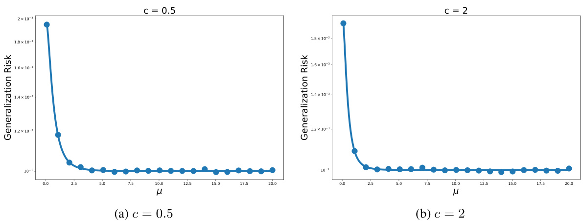
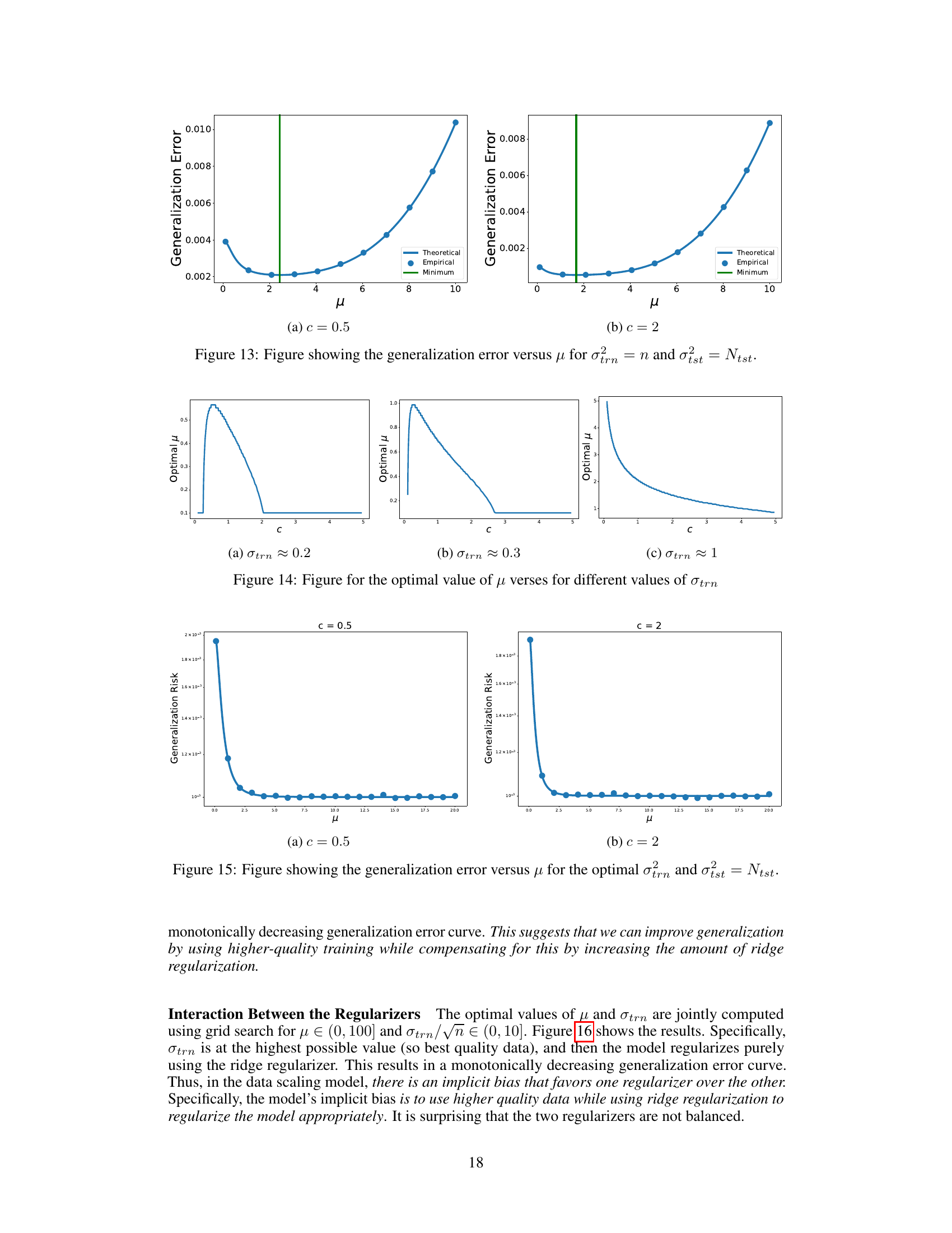
🔼 This figure displays the generalization error versus the training noise standard deviation (σtrn) for two different aspect ratios (c = 0.5 and c = 2) and regularization strengths (μ = 1 and μ = 0.1). The left two subfigures show that there exists an optimal value of σtrn that minimizes the generalization error. The right two subfigures then show the risk when this optimal value of σtrn is used for the data scaling and parameter scaling regimes. These plots show that the optimal value of σtrn is not sufficient to remove double descent.
read the caption
Figure 11: The first two figures show the σtrn versus risk curve for c = 0.5, μ = 1 and c = 2, μ = 0.1 with d = 1000. The second two figures show the risk when training using the optimal σtrn for the data scaling and parameter scaling regimes.

🔼 This figure compares the theoretical risk curve derived from Theorem 1 with empirical results obtained through simulations. Three subfigures are presented, each corresponding to a different value of the regularization parameter μ (0.1, 1, and 2). The data scaling regime is used, where the number of data points (n) is varied while keeping the dimensionality (d) constant at 1000. Each empirical data point in the plots is an average of at least 100 simulation trials. Appendix G provides further details about the experimental setup.
read the caption
Figure 2: Figure showing the theoretical risk curve from Theorem 1 and empirical values in the data scaling regime for different values of μ [(L) μ = 0.1, (C) μ = 1, (R) μ = 2]. Here σtrn = √n, σtst = √ntst, d = 1000, Ntst = 1000. For each empirical point, we ran at least 100 trials. More details can be found in Appendix G.

🔼 This figure compares the theoretical risk curve derived from Theorem 1 with empirical results from simulations for three different values of the regularization parameter μ (0.1, 1, and 2). The data scaling regime is used (n varies, d is fixed), and for each empirical point at least 100 trials were run. The plots show that the theoretical curve accurately captures the double descent phenomenon in the under-parameterized regime.
read the caption
Figure 2: Figure showing the theoretical risk curve from Theorem 1 and empirical values in the data scaling regime for different values of μ [(L) μ = 0.1, (C) μ = 1, (R) μ = 2]. Here σtrn = √n, σtst = √ntst, d = 1000, Ntst = 1000. For each empirical point, we ran at least 100 trials. More details can be found in Appendix G.
Full paper#
