↗ OpenReview ↗ NeurIPS Homepage ↗ Chat
TL;DR#
Deep learning’s success relies heavily on optimization algorithms, despite the complex non-convex nature of its loss landscapes. Existing theoretical analyses often make overly simplistic assumptions, such as the Polyak-Łojasiewicz (PL) inequality, which frequently don’t hold for real-world deep learning models. These assumptions often necessitate unrealistic levels of over-parameterization. This limits the applicability of theoretical findings and hinders the development of more robust optimization techniques.
This paper introduces a new function class characterized by a novel α-β-condition. Unlike previous conditions, this new condition addresses the limitations by explicitly allowing for saddle points and local minima, while not requiring excessive over-parameterization. The authors provide theoretical convergence guarantees for commonly used gradient-based optimizers under the α-β-condition and validate their findings through both theoretical analysis and empirical experiments using various deep learning models, including ResNets, LSTMs, and Transformers. The empirical results demonstrate the practical relevance of the α-β-condition across various architectures and datasets.
Key Takeaways#
Why does it matter?#
This paper is crucial because it offers a novel theoretical framework for understanding deep learning optimization, moving beyond oversimplistic assumptions. It provides convergence guarantees for standard optimizers under a newly proposed condition, validated empirically across diverse models. This opens avenues for more robust and efficient deep learning algorithms.
Visual Insights#

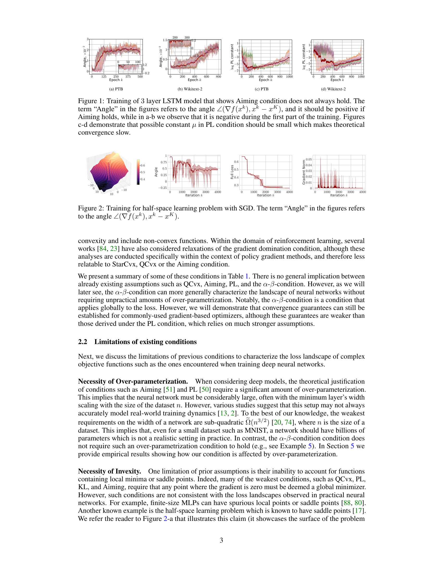
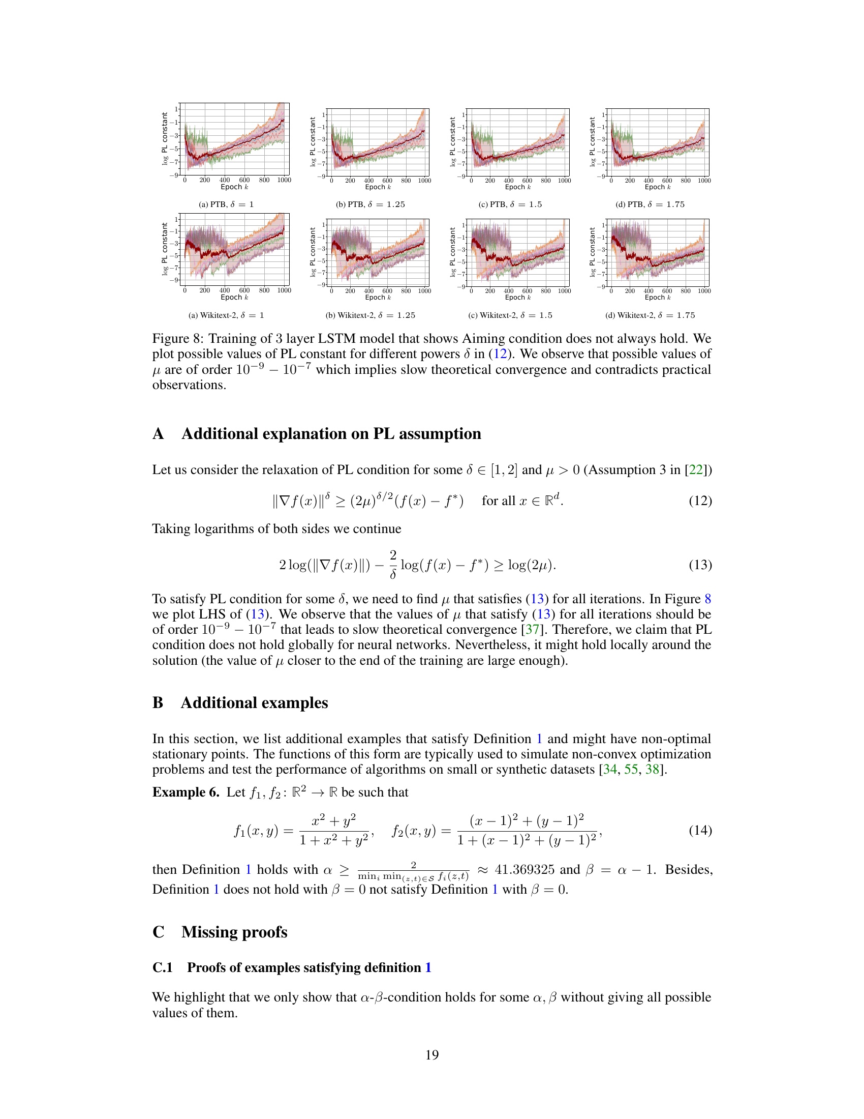
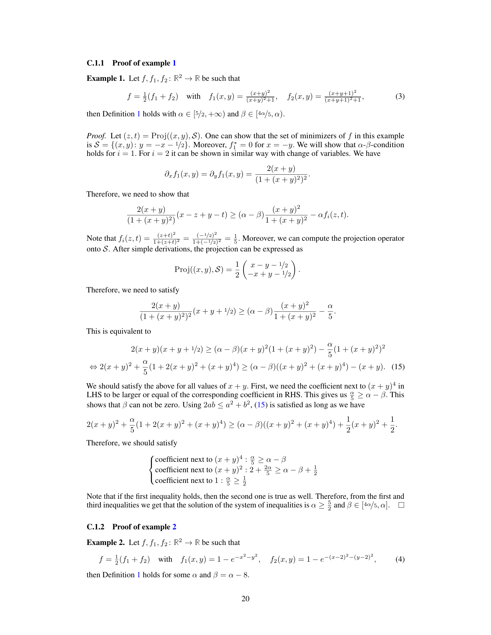
This figure shows the results of training a 3-layer LSTM model on two datasets (PTB and Wikitext-2). The plots illustrate that the Aiming condition, a commonly used assumption in optimization theory, does not always hold during training. Specifically, the angle between the gradient and the direction to the minimum is negative at the beginning of the training process for both datasets. Additionally, the plots show that the Polyak-Łojasiewicz (PL) constant (μ) must be small for the PL condition to hold, resulting in slow convergence, whereas empirical evidence suggests fast convergence. This discrepancy highlights limitations of existing theoretical conditions in characterizing the loss landscape of deep neural networks.

The table summarizes several existing conditions used in optimization, including QCvx, Aiming, and PL, comparing their definitions and limitations. It highlights that these conditions often exclude saddle points and local minima and frequently require impractical levels of over-parametrization for neural networks. In contrast, the newly proposed α-β-condition is designed to address these limitations by characterizing loss landscapes that can include saddle points and local minima without requiring excessive over-parametrization.
In-depth insights#
Loss Landscape#
The concept of a loss landscape is crucial for understanding the optimization process in deep learning. It’s a high-dimensional surface where each point represents a model’s parameters and the height corresponds to the loss function value. The landscape’s shape dictates the difficulty of finding optimal parameters, with smooth landscapes generally being easier to navigate than those with numerous local minima or saddle points. The research delves into the nature of the loss landscape for neural networks without excessive over-parameterization, a condition often assumed in theoretical analyses, but rarely met in practice. It introduces a novel condition (α-β-condition) to effectively characterize this challenging landscape. Unlike previous assumptions, the α-β condition permits saddle points and local minima, which align more closely with empirical observations in practical models. Furthermore, the research establishes theoretical convergence guarantees of gradient-based optimizers under this novel condition, supporting its practical significance and providing a more robust theoretical grounding for understanding the success of deep learning optimization.
α-β Condition#
The proposed \alpha-\beta condition offers a novel perspective on characterizing the loss landscape of neural networks, addressing limitations of existing conditions like Polyak-Łojasiewicz (PL) and Aiming. Unlike previous assumptions that often exclude saddle points and require extensive over-parametrization, \textbf{the \alpha-\beta condition allows for both local minima and saddle points} while potentially needing less over-parameterization. Its theoretical soundness is demonstrated through the derivation of convergence guarantees for various gradient-based optimizers. \textbf{Empirical validation across diverse deep learning models and tasks further supports its practical relevance and effectiveness}. The \alpha-\beta condition’s flexibility in characterizing complex landscapes makes it a valuable tool for analyzing and improving the optimization strategies employed in deep learning, potentially leading to more robust and efficient training methods.
Convergence Rates#
Analyzing convergence rates in optimization algorithms is crucial for understanding their efficiency and effectiveness. The rate at which an algorithm approaches a solution significantly impacts its practical applicability, especially for large-scale machine learning problems. Different algorithms exhibit varying convergence behaviors, depending on factors like the problem’s structure (convexity, smoothness), algorithm parameters (step size, momentum), and the nature of the data. Theoretical analysis often provides bounds on the convergence rate, expressed as a function of the number of iterations or the amount of data processed. These bounds are valuable tools, although they might not always reflect real-world performance due to simplifying assumptions. Empirical evaluations of convergence rates are equally important, complementing theoretical analysis by providing insights into practical behavior in diverse scenarios. The interplay between theoretical analysis and empirical observations helps in gaining a thorough understanding of algorithm performance. Investigating the influence of over-parametrization on convergence rates is also a critical consideration, as it significantly impacts the generalizability and efficiency of the algorithms.
Experimental Setup#
A well-structured ‘Experimental Setup’ section in a research paper is crucial for reproducibility and validation. It should detail the data used, including its source, preprocessing steps, and any relevant characteristics like size and distribution. Specifics about the models employed are key: architecture, hyperparameters (and their selection rationale), and training procedures (optimization algorithm, learning rate schedule, batch size, etc.) must be clearly outlined. Evaluation metrics used to assess model performance should be precisely defined. The setup should also address any potential biases or confounding factors, promoting the trustworthiness of results. A strong emphasis on reproducibility is achieved by including sufficient detail for others to replicate the experiments. This involves documenting the computational environment and software versions, to prevent discrepancies due to variations in these elements. Transparency and clarity are paramount: the description must be explicit and accessible to a broad scientific audience. This allows readers to critically evaluate the methodology, interpret the findings accurately, and potentially extend the research. Furthermore, a thorough setup minimizes ambiguity and helps to understand limitations of the work, leading to more impactful and robust conclusions.
Future Work#
The paper’s lack of a dedicated ‘Future Work’ section is notable. However, the conclusion hints at several promising avenues. Extending the theoretical convergence analysis to encompass more sophisticated optimizers like Adam and incorporating momentum into the analysis are key directions. Empirically validating the α-β condition across a wider range of network architectures and datasets, including those with significantly different levels of over-parameterization, would strengthen the findings. Exploring the impact of various initialization strategies on satisfying the α-β condition is another area meriting investigation. Finally, further probing the relationship between the α-β condition and other existing landscape characterizations, such as the Polyak-Łojasiewicz inequality, warrants deeper exploration to reveal a more complete picture of the loss landscape of modern neural networks. This exploration will help to improve our understanding of their optimization properties.
More visual insights#
More on figures

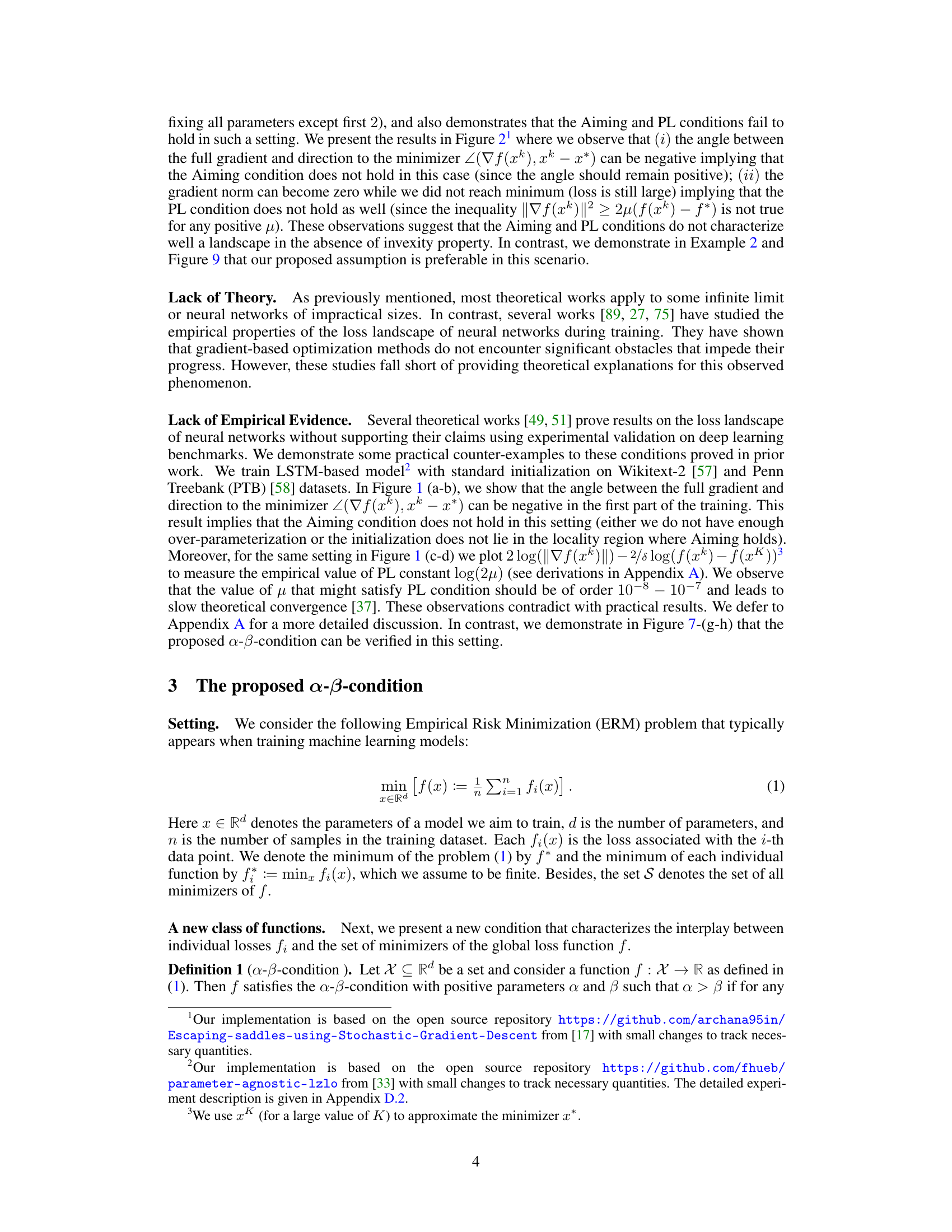
This figure shows the training process of a half-space learning problem using SGD. It contains four subfigures that illustrate various aspects of the optimization process. The ‘Angle’ refers to the angle between the gradient and the direction to the minimizer (∠(∇f(xk), xk − xK)). The plots showcase the angle over iterations, the full loss, the gradient norm, and the evolution of the angle over time. The half-space learning problem is known to have saddle points, and the figure seems to demonstrate the behavior of the optimizer in navigating this complex loss landscape.

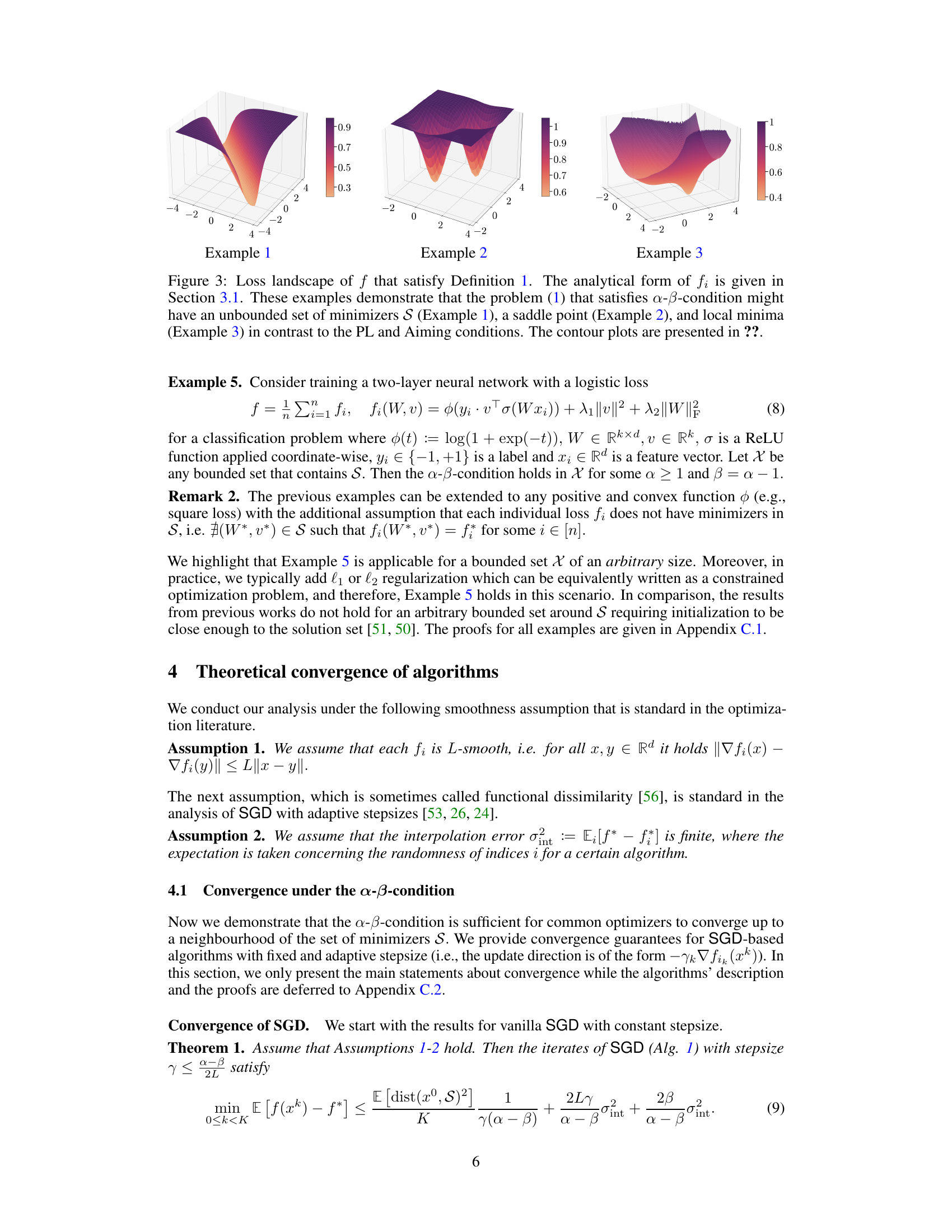
This figure shows the loss landscape of three example functions that satisfy the α-β condition, illustrating that the α-β condition can capture functions with an unbounded set of minimizers, saddle points, and local minima, unlike other conditions like PL and Aiming.

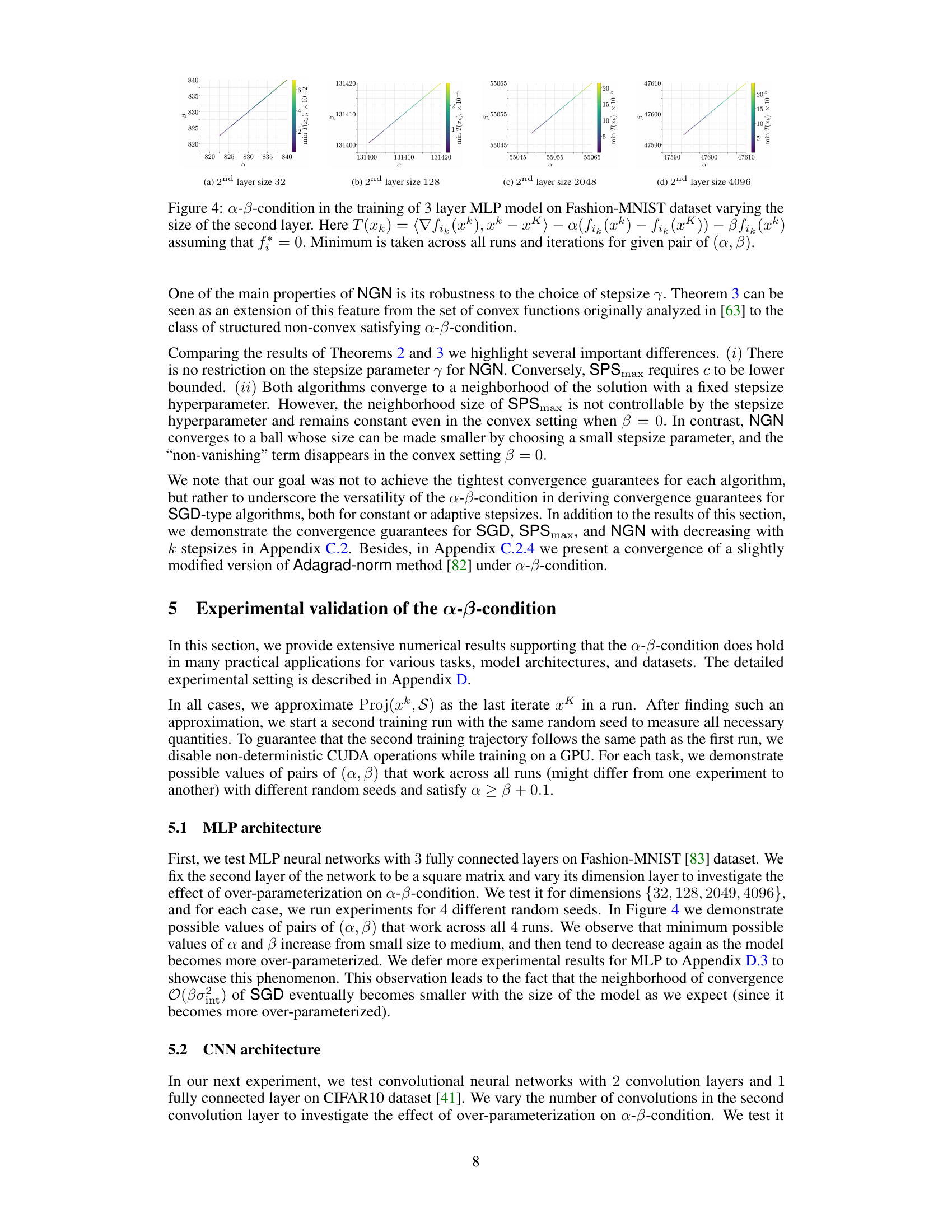
The figure shows the α-β-condition during the training of a 3-layer MLP model on the Fashion-MNIST dataset. The size of the second layer is varied to investigate the effect of over-parametrization on the α-β-condition. The plots show the minimum value of T(xk) across all runs and iterations for given pairs of (α, β). The results show that the minimum possible values of α and β increase from small sizes to medium sizes and then decrease as the model becomes more over-parametrized.

This figure displays the values of α and β parameters obtained during the training of a Convolutional Neural Network (CNN) model on the CIFAR-10 dataset. The x-axis represents the number of convolutions in the second layer of the CNN. The y-axis shows the minimum values of α and β parameters obtained across all runs and iterations during training, where these parameters satisfy the α-β-condition (a newly proposed condition in the paper) with α > β. The different subplots correspond to different numbers of convolutions, illustrating the relationship between model over-parameterization (as indicated by increasing convolution count) and the values of the α and β parameters required to satisfy the α-β-condition.

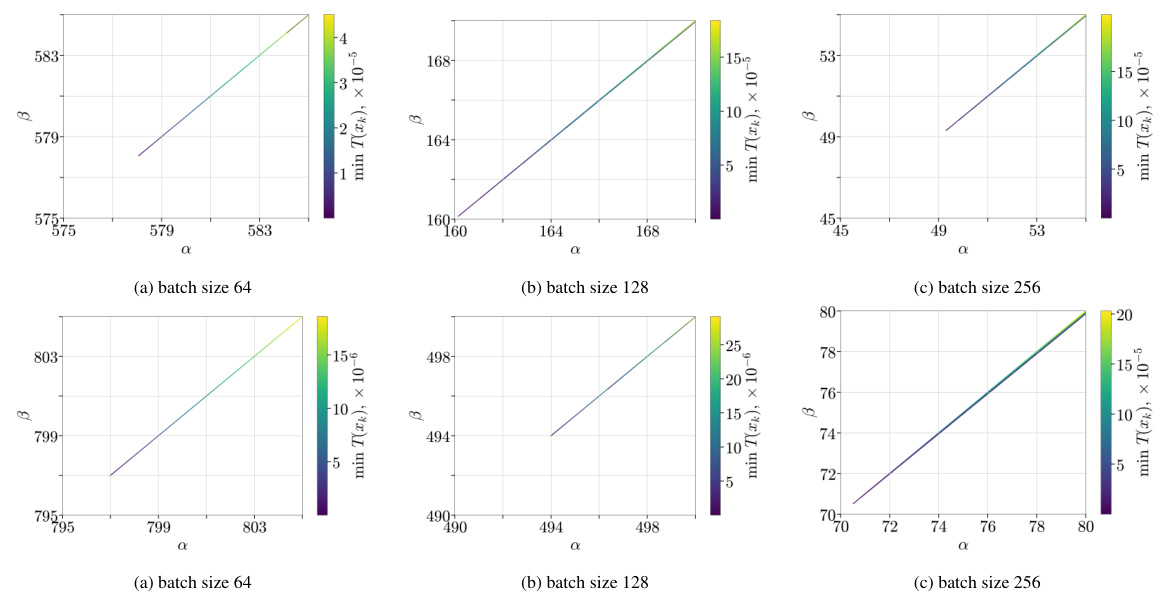
This figure displays the results of an experiment evaluating the α-β-condition on the training of a Resnet9 model using the CIFAR100 dataset. The experiment varied the batch size during training. The plot shows the minimum value of the expression T(x) = (∇fik (xk), xk – xK) – α(fik (xk) – fik (xK)) – β fik (xk) across all runs and iterations for each pair of α and β values. The value of f* is assumed to be 0. This illustrates how the α-β-condition holds under different batch sizes in this setting.

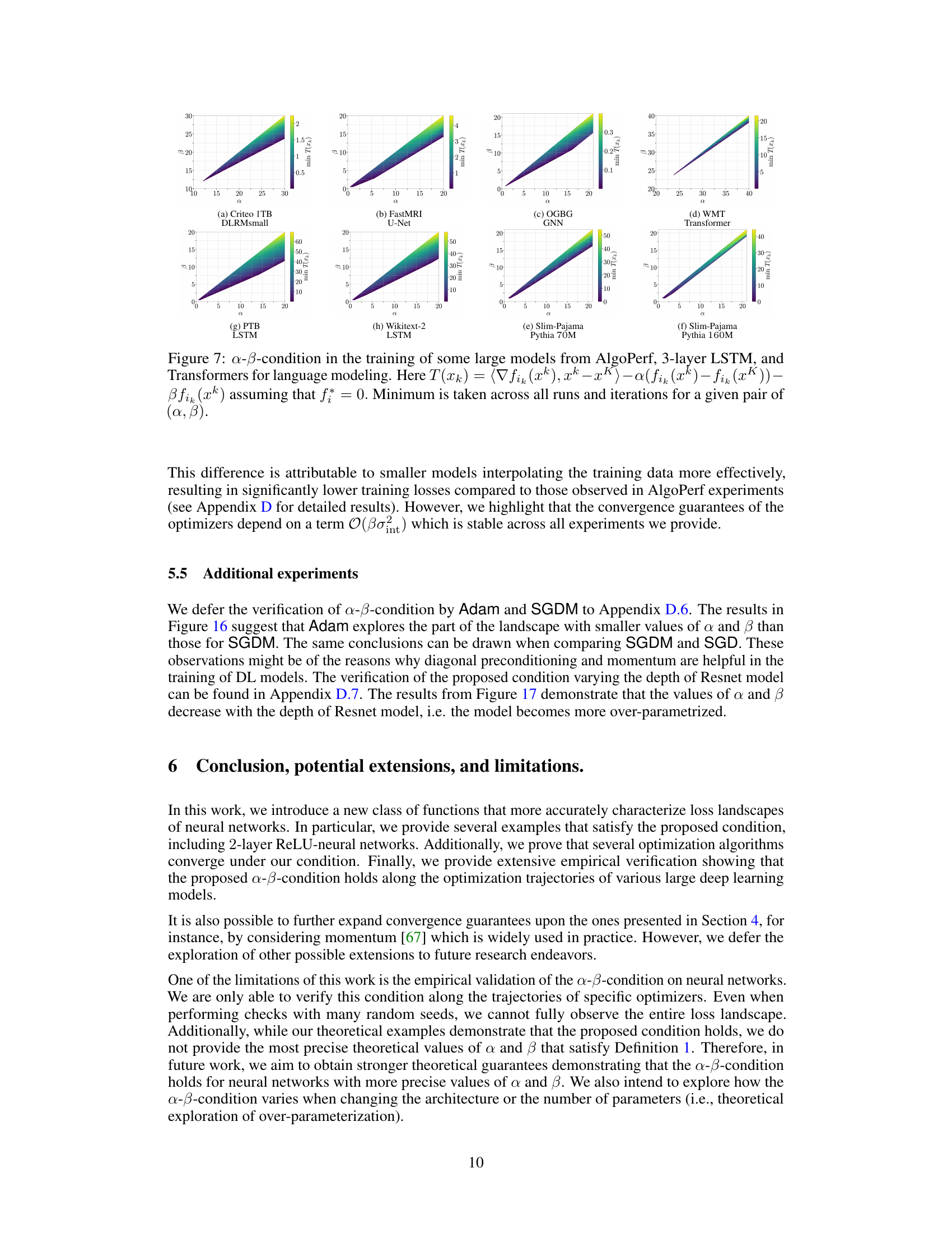
This figure displays the results of applying the α-β-condition to several large language models and other deep learning models during training. It shows how the angle between the gradient and the projection onto the set of minimizers varies across different models. The heatmaps illustrate the minimum values of α and β that satisfy the α-β-condition for each model across multiple training runs and iterations. The results demonstrate the applicability of the α-β-condition to a diverse range of architectures and problem settings.
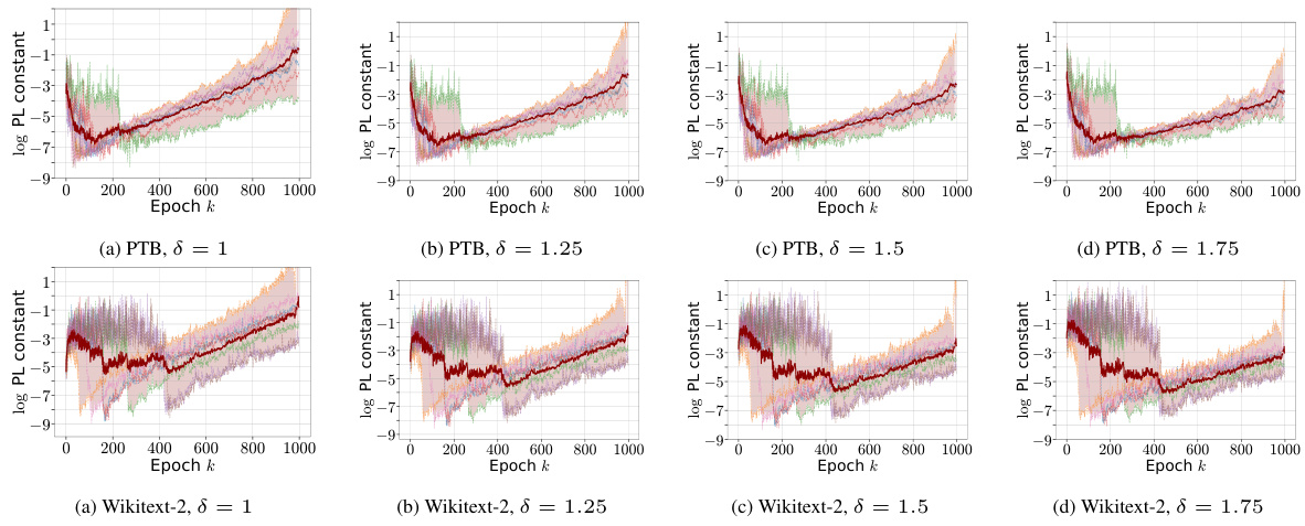
This figure shows the result of training a 3-layer LSTM model on PTB and Wikitext-2 datasets. It demonstrates that the widely recognized Polyak-Łojasiewicz (PL) inequality, often used to guarantee convergence in optimization, is not always satisfied in practice. The plots show that the possible values for the PL constant μ are very small (around 10^-9 to 10^-7), which implies slow convergence according to theoretical analysis. This contrasts with the observed fast convergence in practice. The figure visualizes the inadequacy of PL inequality for characterizing the loss landscape of deep neural networks without significant over-parametrization, motivating the need for the new α-β-condition proposed in the paper.

This figure shows the results of training a model on a half-space learning problem using SGD. It displays multiple plots illustrating various aspects of the training process. The plot labeled ‘Angle’ shows the angle between the gradient and the direction to the minimizer. This angle should be positive if the ‘Aiming’ condition (a known condition used for convergence analysis) holds, and the figure shows how it does not always hold. The plot labeled ‘Full Loss’ shows the loss function, highlighting how it is decreasing as training progresses. The ‘Gradient Norm’ plot shows the norm of the gradient, which indicates the magnitude of changes in the loss function. The plot labeled ‘min T(xk)’ shows the minimum value of a particular function T(xk), which is a measure relevant to the newly introduced α-β condition proposed in the paper. The figure demonstrates that while the Aiming condition doesn’t always hold, the α-β condition, proposed in the study, does provide a better characterization of the optimization landscape.
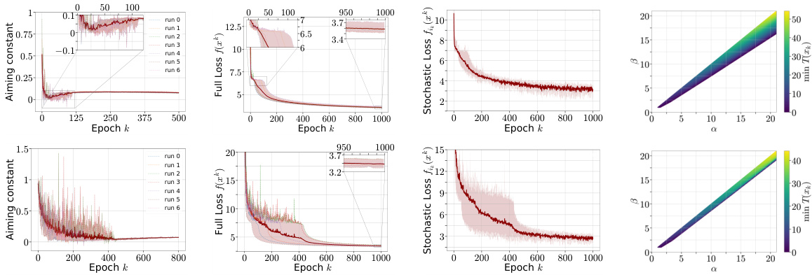
The figure shows the training process of a 3-layer LSTM model on two datasets: Penn Treebank (PTB) and WikiText-2. It visualizes how the Aiming condition (a measure of gradient alignment with the direction to the minimizer) and the Polyak-Łojasiewicz (PL) condition (a measure of the relationship between gradient norm and function value) behave during training. The plots include the Aiming coefficient, full loss, stochastic loss, and the PL constant. The goal is to show whether the Aiming and PL conditions, commonly used to analyze optimization algorithms, hold throughout the training process in these models. Note that the term ‘Angle’ refers to the angle ∠(∇f(xk), xk – xK).

This figure shows the values of α and β parameters of the α-β condition during the training process of a 3-layer MLP model on the Fashion-MNIST dataset. The x-axis represents α, the y-axis represents β, and different subfigures show results for different sizes of the second layer (32, 128, 512, 1024, 2048, 4096). The color intensity represents the minimum value of T(xk) across all iterations and runs, where T(xk) is a function of the gradient and the distance to the minimizer, α and β. The figure aims to illustrate how the α-β condition parameters change during the training, and how these changes are related to the over-parameterization of the model.

The figure shows the values of α and β parameters for the α-β-condition during the training of a 3-layer MLP model on the Fashion-MNIST dataset. The size of the second layer is varied to investigate the effect of over-parameterization. The plot shows that minimum possible values of α and β increase from small size to medium, and then tend to decrease again as the model becomes more over-parametrized. This observation leads to the fact that the neighborhood of convergence O(βσnt) of SGD eventually becomes smaller with the size of the model.
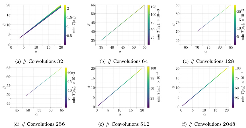
This figure shows the values of α and β parameters obtained during the training of a 3-layer Multilayer Perceptron (MLP) model on the Fashion-MNIST dataset. The size of the second layer was varied to investigate the effect of over-parameterization on the α-β condition. The plot shows how the minimum possible values of α and β change with the size of the second layer. It suggests that the minimum values increase initially with size, but start decreasing as the model becomes over-parametrized, leading to smaller neighborhood size O(βσint).
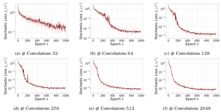
The figure shows the training curves of stochastic loss for a 3-layer MLP model trained on the Fashion-MNIST dataset. The x-axis represents the training epoch, and the y-axis represents the stochastic loss. Multiple lines are shown, each corresponding to a different size of the second layer of the MLP model. The goal is to observe how the loss changes depending on the model’s width to investigate the effect of over-parameterization on the α-β condition.

The figure shows the training curves of ResNet9 model trained on CIFAR100 dataset with different batch sizes (64, 128, 256, and 512). Each curve represents the stochastic loss over epochs. The aim is to illustrate how the minimum value of the stochastic loss changes with the batch size. It shows that the minimum stochastic loss increases with the batch size, which indicates that the model is further from being over-parameterized as the batch size increases.
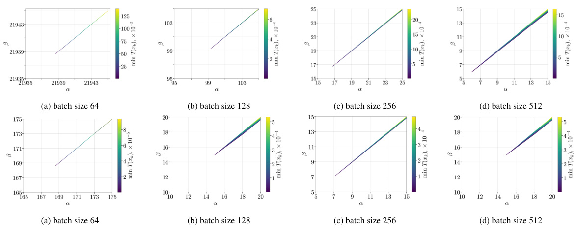
The figure shows the values of α and β parameters during the training process of a 3-layer Multilayer Perceptron (MLP) model on the Fashion-MNIST dataset. The x-axis represents the size of the second layer, while the y-axis displays the minimum values of α and β that satisfy the α-β condition, which is a novel condition proposed in the paper. The results suggest a relationship between the model’s over-parametrization (second layer size) and the minimum α and β values that satisfy the α-β condition. The minimum possible values of α and β first increase with the second layer size (indicating a more complex landscape) but then begin to decrease as the model becomes more over-parameterized, suggesting that a simpler loss landscape is observed with significant over-parametrization.
This figure displays the results of an experiment assessing the α-β condition during the training of a 3-layer Multilayer Perceptron (MLP) model on the Fashion-MNIST dataset. The experiment varies the size of the second layer of the MLP to investigate the impact of over-parameterization on the α-β condition. The plot shows the minimum value of the expression T(xk) = (∇fik (xk), xk – xK) – a(fik (xk) – fik (xK)) – ẞfik (xk) across all runs and iterations, for given values of α and β. The minimum is taken to check if the α-β condition holds at any point during training. The results are shown for different sizes of the second layer (32, 128, 2048, and 4096), providing insights into how the α-β condition is affected by over-parameterization.

The figure shows the training curves of several large models from the AlgoPerf benchmark. Each subfigure displays the stochastic loss over training iterations for a specific model and dataset, with multiple runs shown for each model to illustrate variability. This provides empirical evidence for the α-β-condition.

This figure shows the training statistics for Pythia language models with different sizes (70M and 160M) trained on the SlimPajama dataset. The plots show stochastic loss and perplexity for three different runs, visualizing the training progress and stability.
More on tables

This table summarizes several existing conditions used in optimization, including QCvx, Aiming, PL, and the newly proposed α-β-condition. It compares their definitions, limitations, and how they relate to the loss landscape of neural networks. The α-β-condition is highlighted for its ability to handle saddle points and local minima without requiring extensive over-parametrization, a major limitation of other methods.

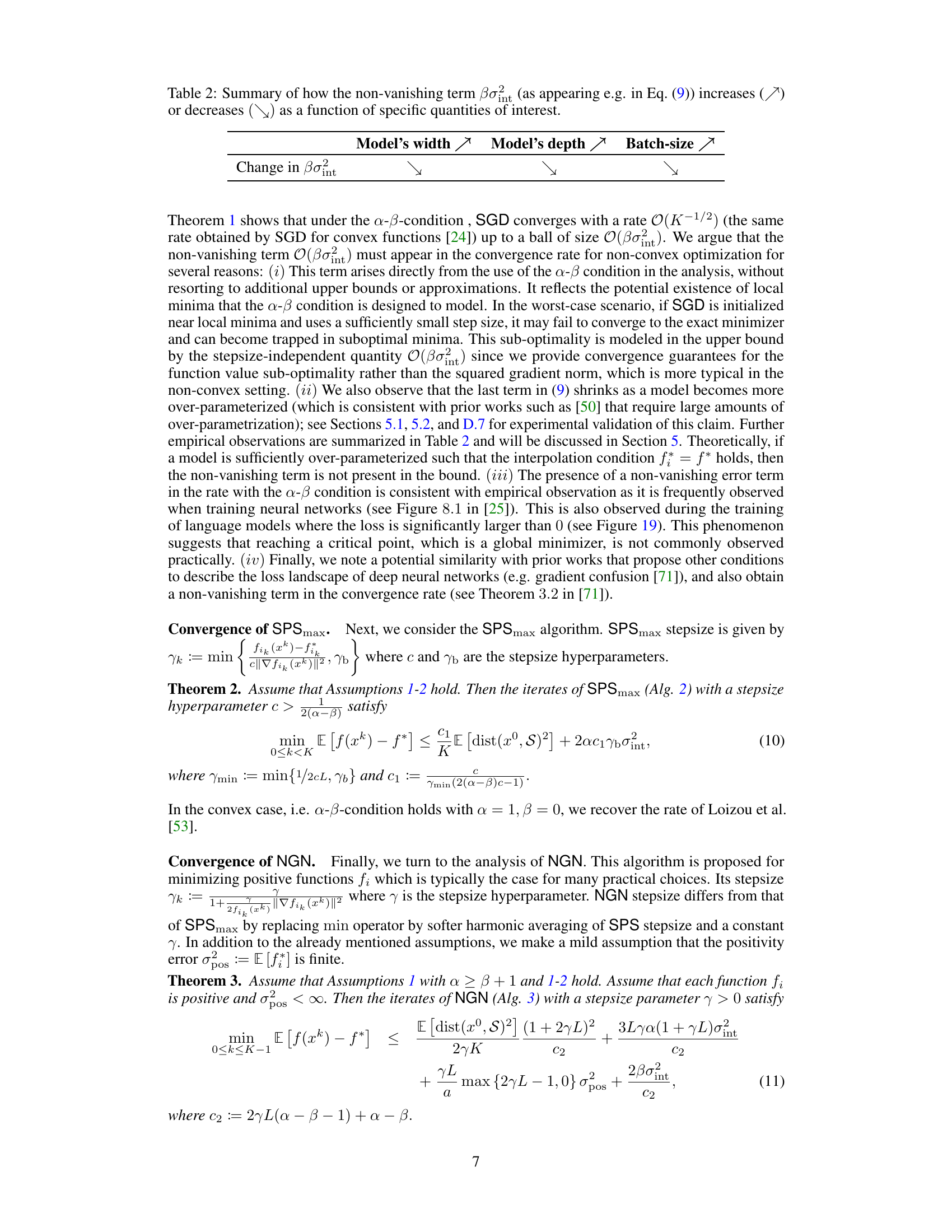
This table shows how the non-vanishing term βσint in the convergence rate changes depending on the model’s width, depth, and batch size. It summarizes empirical observations regarding the impact of model architecture choices on the convergence guarantees derived using the α-β-condition. The symbol √ indicates a decrease in the term, while 2 indicates an increase.
Full paper#


