TL;DR#
Many machine learning methods rely on embedding data into a low-dimensional vector space. This paper focuses on determining the minimum embedding dimension needed to accurately capture distance relationships within datasets. The authors tackle this problem in two scenarios: contrastive learning and k-nearest neighbor (k-NN) search. Both involve comparing distances between points, but with different types of information. A key challenge is that directly preserving all distance information often requires high dimensionality.
The study leverages the concept of graph arboricity to derive tight bounds on embedding dimensions for both contrastive learning and k-NN in various lp-spaces. For instance, it shows that preserving the relative order of nearest neighbors in l2 space only requires O(k) dimensions. This work introduces novel theoretical frameworks and analytical tools to understand embedding dimensionality, offering practical guidance for model development and optimization in machine learning.
Key Takeaways#
Why does it matter?#
This paper significantly advances our understanding of embedding dimensionality in contrastive learning and k-NN, offering both theoretical bounds and practical guidance. It’s crucial for researchers designing efficient deep learning architectures and optimizing model performance. The results directly impact the selection of embedding dimensions, leading to more efficient and effective models. The introduction of graph arboricity as a key analytical tool opens new avenues for research in related fields.
Visual Insights#

🔼 This figure illustrates how the embedding vector for a node (x4) is constructed based on the embedding vectors of its preceding neighbors (x1, x2, x3) in the constraint graph. The inner product between the embedding vectors of connected nodes is set to be equal to the rank of the edge connecting them, ensuring that the distance between the nodes reflects their relative importance according to the edge weights.
read the caption
Figure 2: Example construction of ✰. The embedding ✰4 is computed based on the embeddings of its already processed neighbors ✰1, ✰2, ✰3. We find the solution ✰4 to the linear system so that, for each edge to a preceding neighbor, the inner product equals the rank of the edge.

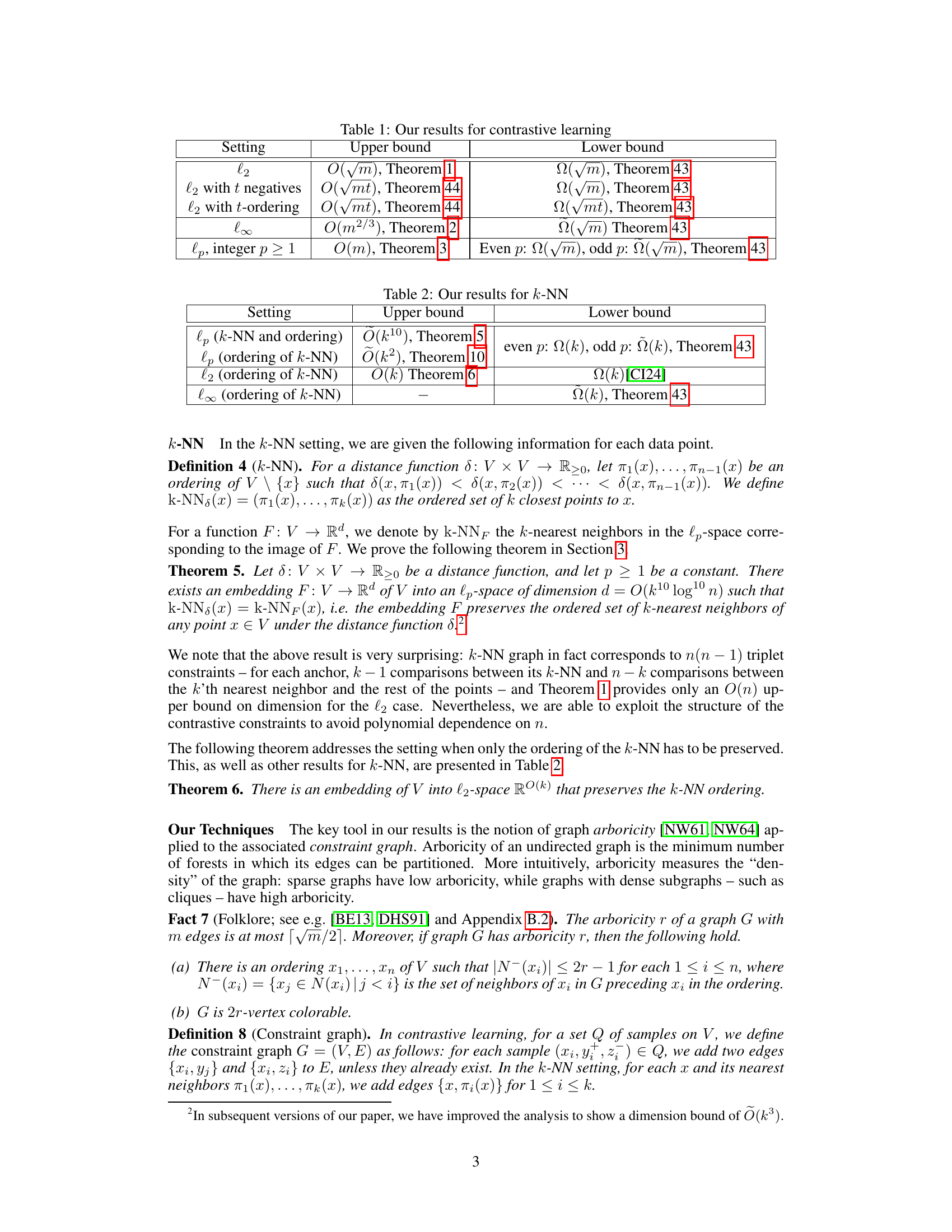
🔼 This table summarizes the upper and lower bounds on the embedding dimension for contrastive learning in different lp spaces (l2, l∞, lp for integer p ≥ 1). It shows the results for three settings: l2, l2 with t negatives, and l2 with t-ordering. The upper bounds are derived from Theorems 1, 2, and 3 in the paper, while the lower bounds are from Theorem 43. The table highlights the dependence of the embedding dimension on the number of samples (m) and the number of negative examples (t).
read the caption
Table 1: Our results for contrastive learning
In-depth insights#
Embedding Space#
The concept of “Embedding Space” in the context of contrastive learning and k-Nearest Neighbors (k-NN) is central to the paper’s investigation. The authors explore the dimensionality (or dimension) of this space, aiming to find the smallest embedding dimension needed to effectively represent data while preserving crucial relationships. This is crucial as lower dimensions simplify computation and improve model efficiency. They demonstrate that the arboricity of the associated graphs (constraint graphs) – representing relationships between data points – plays a significant role in determining this minimal dimension. Tight bounds are derived for l2-space, indicating a direct relationship between embedding dimension and the square root of the number of samples in contrastive learning. For k-NN, the relationship is tied to the value of k, again highlighting the trade-off between dimensionality and the preservation of neighborhood structure. The study’s implications are significant for machine learning architecture design, as choosing appropriate embedding dimensions directly impacts computational cost and model performance.
Contrastive Bounds#
A hypothetical section titled “Contrastive Bounds” in a research paper would likely explore the limits and capabilities of contrastive learning methods. It could delve into theoretical analyses, proving lower and upper bounds on the performance of contrastive learning models under varying conditions (e.g., dataset size, dimensionality, number of negative samples). The focus might be on establishing theoretical guarantees of how well contrastive learning can perform a given task, potentially highlighting the impact of hyperparameters on these bounds. Experimental validation would be crucial, comparing empirical results to the predicted bounds to assess the accuracy of the theoretical models. The discussion could extend to the relationship between contrastive learning bounds and generalization capabilities, examining whether tighter bounds correlate with better generalization performance. Overall, a “Contrastive Bounds” section would offer a rigorous examination of the theoretical underpinnings of contrastive learning, aiming to provide a deeper understanding of its strengths and limitations.
k-NN Ordering#
The k-NN ordering problem, a crucial aspect of this research, focuses on preserving the relative ordering of each data point’s k-nearest neighbors (k-NN) after embedding the data into a lower-dimensional space. The paper investigates the minimum embedding dimension required to maintain this ordering. A key finding is the strong dependence of this dimension on the value of k, suggesting that maintaining the order of closer neighbors is significantly easier than preserving the ordering for more distant points. The analysis leverages the notion of graph arboricity, a measure of graph sparsity, establishing a direct relationship between the arboricity of the k-NN graph and the required embedding dimension. This connection implies that the structure of the k-NN relationships inherently impacts the difficulty of dimensionality reduction while maintaining ordering. The paper also explores the trade-off between preserving the order of k-NNs and preserving k-NNs themselves as nearest neighbors in the reduced space, highlighting the increased dimensionality needed for the latter task. Tight bounds on the embedding dimension are derived for various lp-spaces, demonstrating a theoretical framework with experimental validation on image datasets.
Arboricity Role#
The concept of arboricity plays a crucial role in the paper’s analysis of embedding dimensionality. Arboricity, representing the minimum number of forests needed to partition a graph’s edges, provides a powerful measure of graph density. The authors cleverly leverage this concept to establish tight bounds on the embedding dimension for both contrastive learning and k-NN settings. By relating the arboricity of the constraint graph (representing distance relationships within the data) to the embedding dimension, they demonstrate that sparse datasets (low arboricity) require significantly lower-dimensional embeddings compared to dense datasets. This finding offers crucial insights into the efficiency of embedding techniques and highlights the significance of graph structure in determining embedding complexity. The arboricity-based approach provides a unified framework for analyzing embedding dimensionality across different data representations, paving the way for improved efficiency in various machine learning tasks.
Future Research#
Future research directions stemming from this work on embedding dimensions could explore several avenues. Tightening the bounds presented, particularly the gap between upper and lower bounds, is crucial. This could involve investigating more sophisticated graph-theoretic properties beyond arboricity or developing novel embedding techniques specifically tailored to the structure of contrastive learning or k-NN graphs. Another key area is to investigate the impact of different loss functions and training procedures on embedding dimensions. Extending the theoretical framework to other distance metrics and norm spaces beyond the lp norms is also a promising area. The current work primarily focuses on exact preservation of distances or orderings; relaxing these constraints to allow for approximate preservation with provable guarantees would lead to more practical applications. Finally, further empirical studies on large-scale datasets to validate the theoretical findings and explore the interplay between embedding dimensionality, sample size, and model generalization are essential.
More visual insights#
More on figures
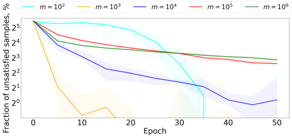
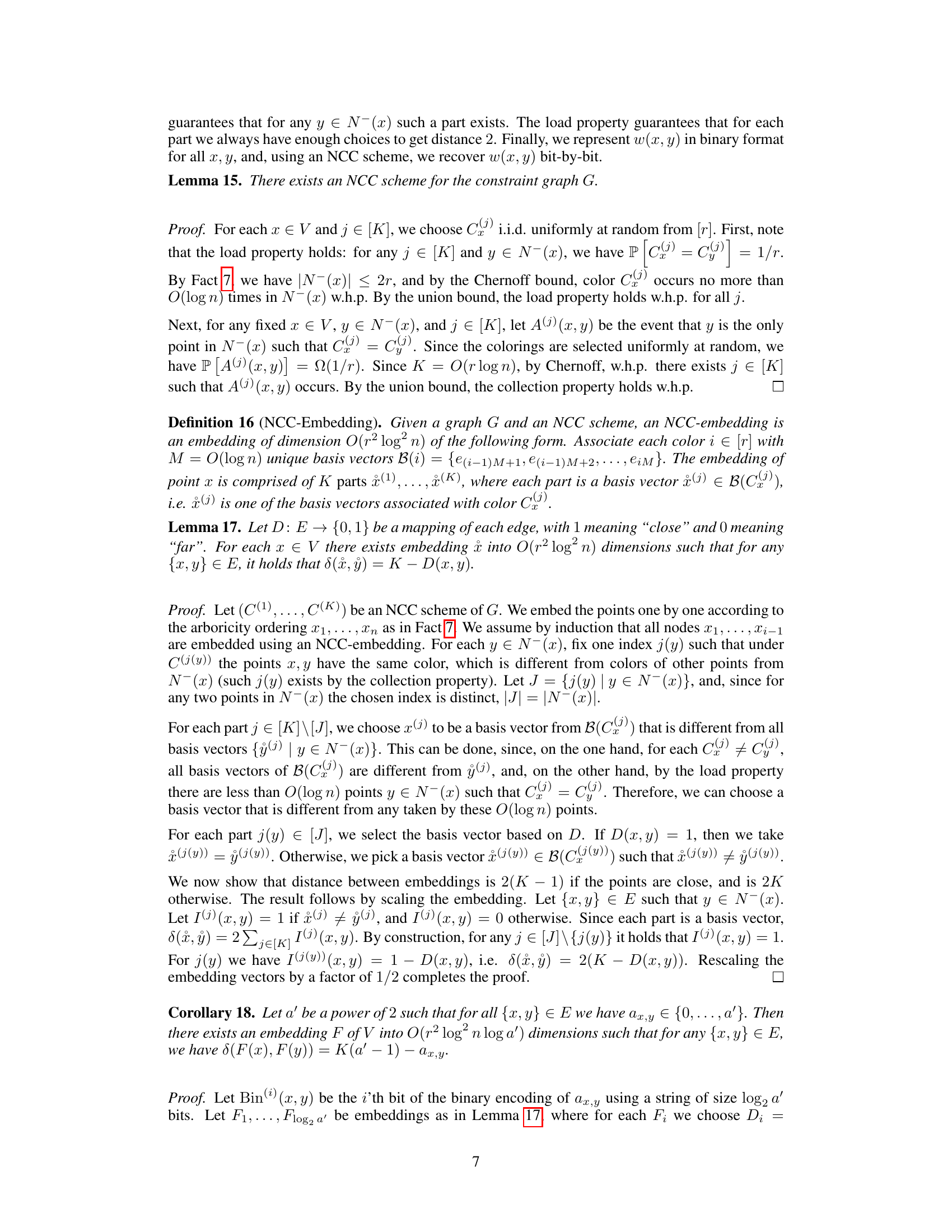
🔼 The figure shows the results of the CIFAR-10 and CIFAR-100 experiments, showing the fraction of unsatisfied samples over training epochs for different numbers of samples (m) and embedding dimensions (d). The shaded areas represent the minimum and maximum values across five runs, illustrating the variability of the results. It visually demonstrates the relationship between the number of samples, embedding dimension, and the success of contrastive learning.
read the caption
Figure 4: Experiments on CIFAR-10 (left) and CIFAR-100 (right). The data points show the average over 5 runs, and the shaded area shows the minimum and the maximum values over the runs
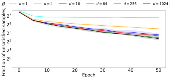
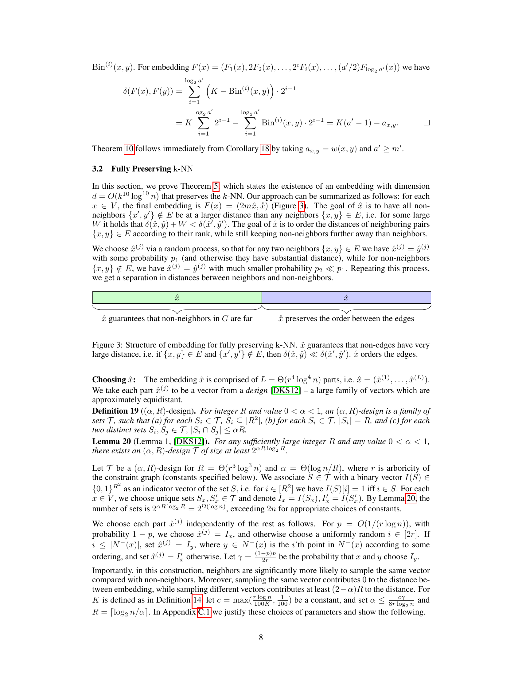
🔼 This figure presents the results of experiments conducted on CIFAR-10 and CIFAR-100 datasets to evaluate the performance of contrastive learning with varying embedding dimensions. The plots show the fraction of unsatisfied samples over epochs for different embedding dimensions (d = 1, 4, 16, 64, 256, 1024). The shaded regions represent the minimum and maximum values across five runs, illustrating variability in the results. The results suggest a relationship between embedding dimension and the accuracy of contrastive learning.
read the caption
Figure 4: Experiments on CIFAR-10 (left) and CIFAR-100 (right). The data points show the average over 5 runs, and the shaded area shows the minimum and the maximum values over the runs

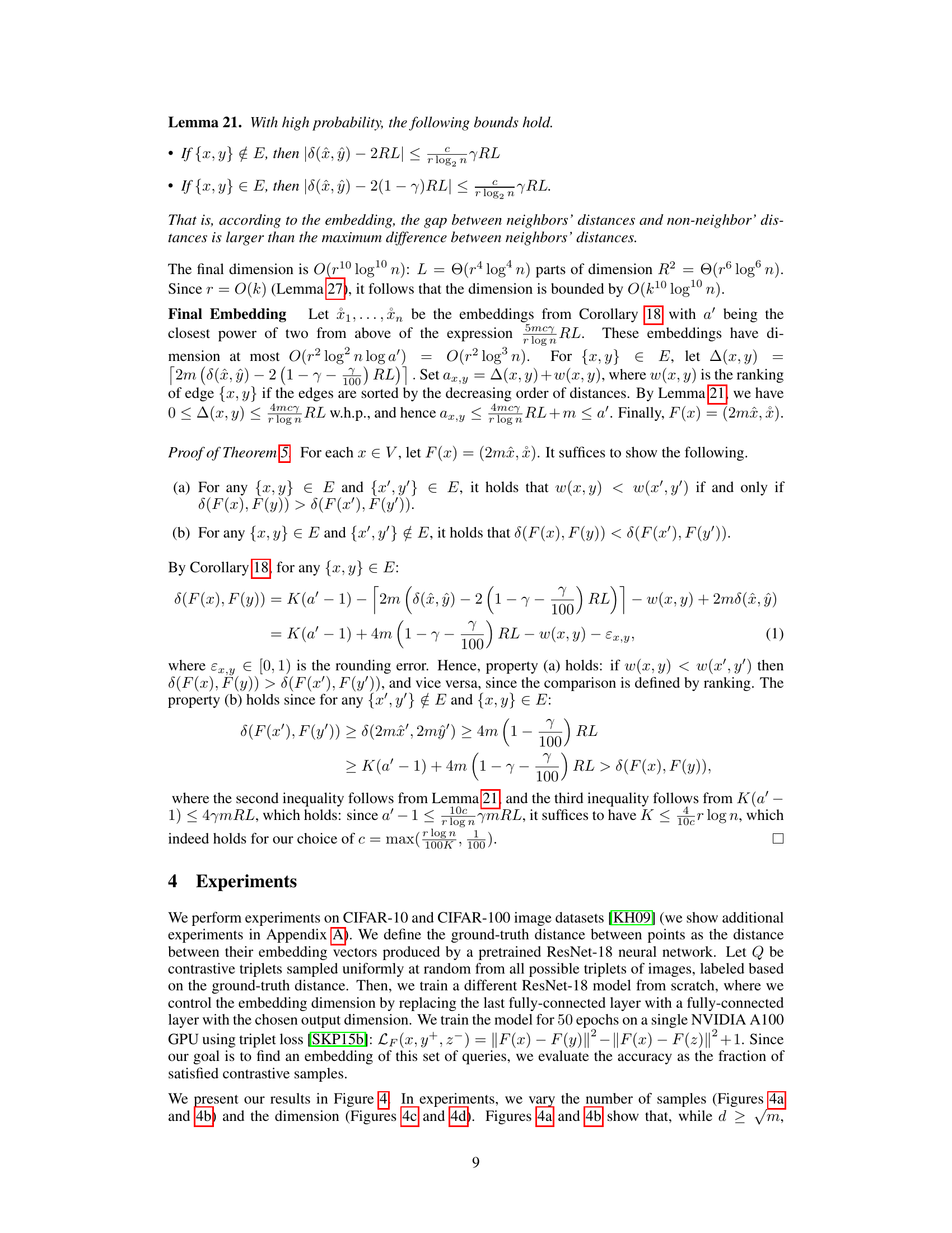
🔼 This figure visualizes the results of experiments conducted on CIFAR-10 and CIFAR-100 datasets to evaluate the impact of the number of samples and embedding dimension on the accuracy of contrastive learning. The plots show the fraction of unsatisfied samples (error rate) over training epochs for varying numbers of samples (m) and embedding dimensions (d). The shaded regions represent the minimum and maximum values across five runs, illustrating the variability of the results.
read the caption
Figure 4: Experiments on CIFAR-10 (left) and CIFAR-100 (right). The data points show the average over 5 runs, and the shaded area shows the minimum and the maximum values over the runs

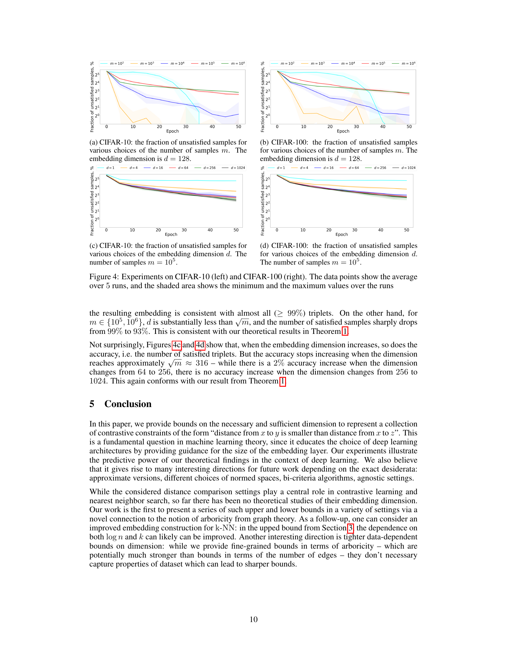
🔼 This figure presents the results of experiments conducted on CIFAR-10 and CIFAR-100 datasets to evaluate the impact of the number of samples and embedding dimension on the accuracy of contrastive learning. The plots show the fraction of unsatisfied samples over training epochs for various settings. The shaded regions indicate the variability across multiple runs of the experiments.
read the caption
Figure 4: Experiments on CIFAR-10 (left) and CIFAR-100 (right). The data points show the average over 5 runs, and the shaded area shows the minimum and the maximum values over the runs
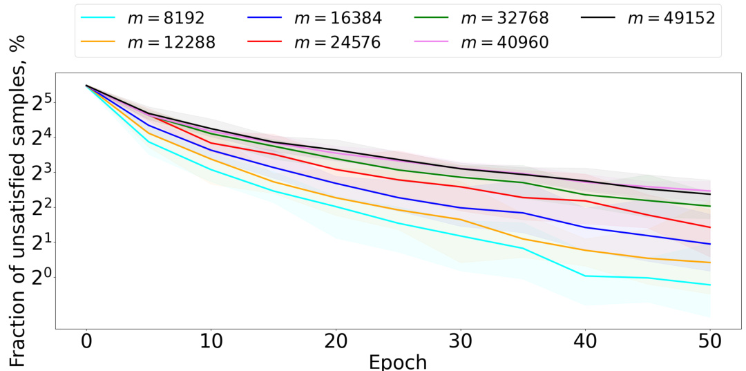
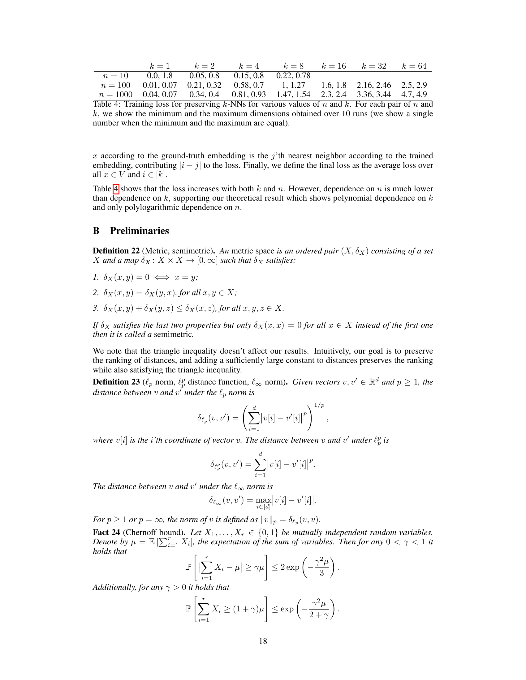
🔼 The figure shows the training accuracy on CIFAR-100 dataset for various values of m. The embedding dimension is fixed at 128. It supports the theoretical result that √m dimensions are required to preserve contrastive samples. For m ≤ d²/2 (where d is the embedding dimension), accuracy is near perfect (99%). Accuracy starts decreasing when m > d²/2.
read the caption
Figure 5: CIFAR-100: the fraction of unsatisfied samples for various choices of the number of samples m. The embedding dimension is d = 128.
More on tables

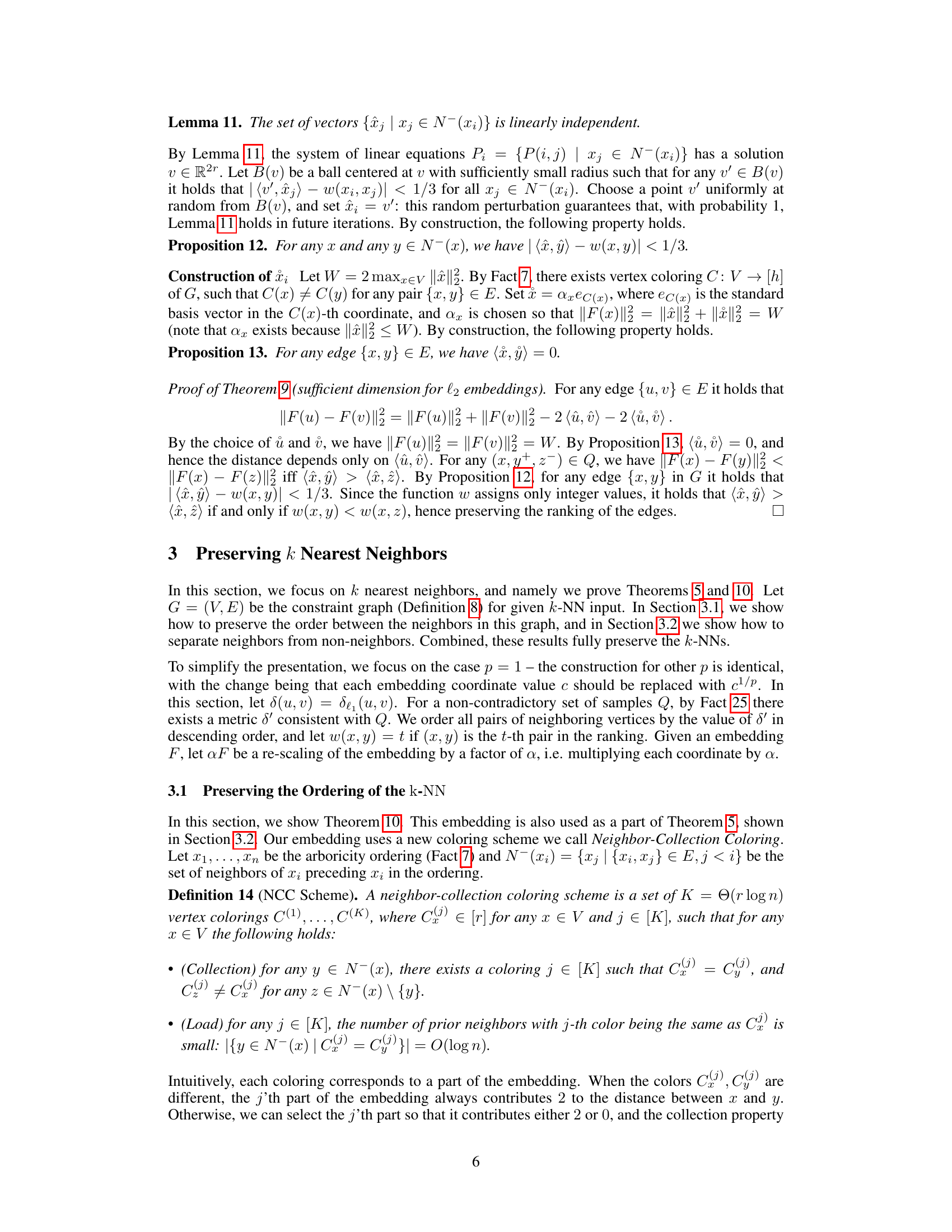
🔼 This table summarizes the upper and lower bounds on the embedding dimension d required to preserve k-nearest neighbor (k-NN) information in different lp-spaces. It shows results for two scenarios: when the exact k-NN must be preserved, and when only the ordering of the k-NN needs to be preserved. The upper bounds represent the sufficient dimension proven in the paper, while the lower bounds represent the necessary dimension. The table demonstrates that the required dimension depends on the type of lp-space used and the strength of the k-NN preservation requirement.
read the caption
Table 2: Our results for k-NN

🔼 This table summarizes the upper and lower bounds on the embedding dimension for contrastive learning in different settings. The settings include the use of l2, l∞, and lp spaces (where p is an integer greater than or equal to 1), with variations in the number of negative samples and whether the ordering of the negative samples is considered.
read the caption
Table 1: Our results for contrastive learning

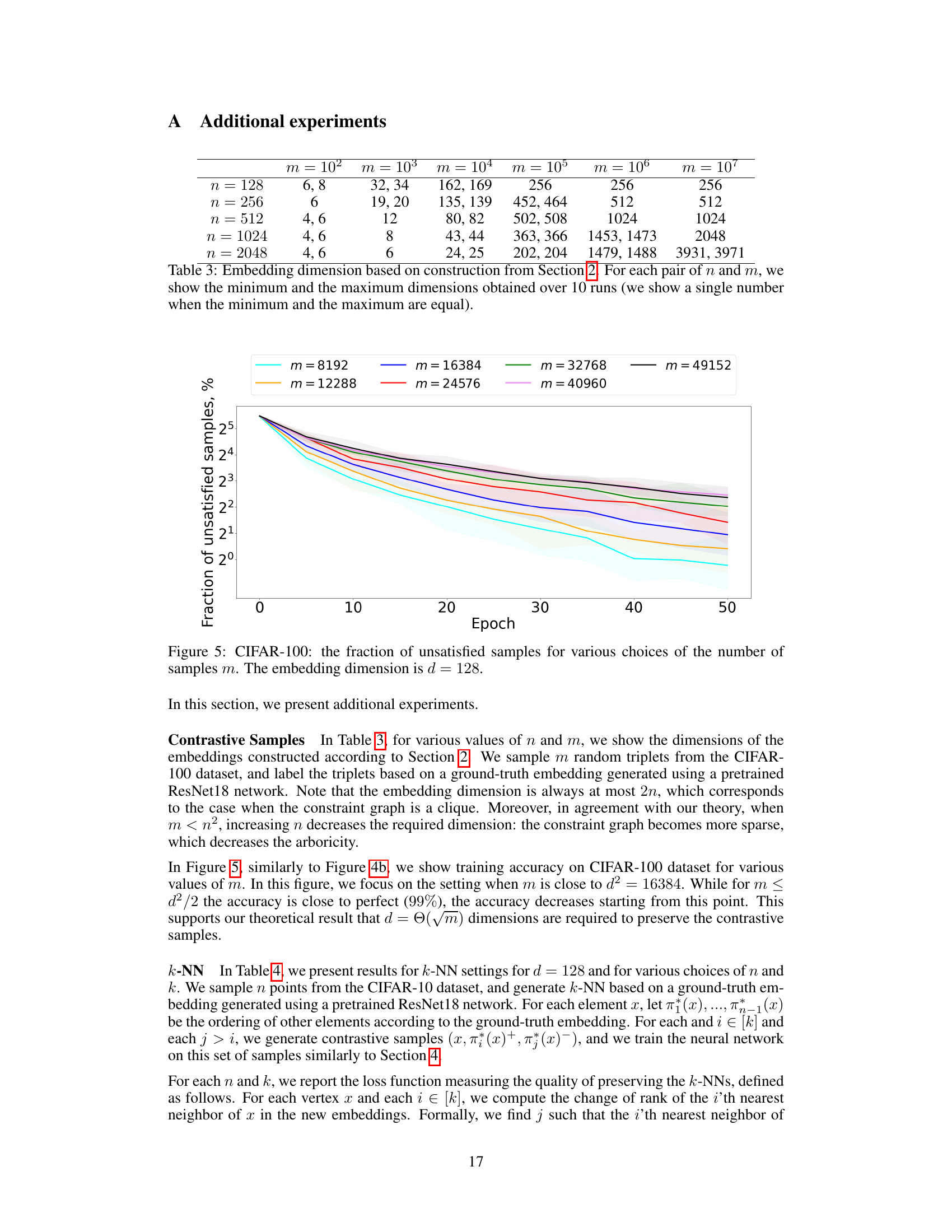
🔼 This table shows the embedding dimensions obtained using the construction from Section 2 of the paper. The minimum and maximum dimensions are shown for various dataset sizes (n) and numbers of contrastive samples (m), giving insights into how the required embedding dimension scales with these factors.
read the caption
Table 3: Embedding dimension based on construction from Section 2. For each pair of n and m, we show the minimum and the maximum dimensions obtained over 10 runs (we show a single number when the minimum and the maximum are equal).

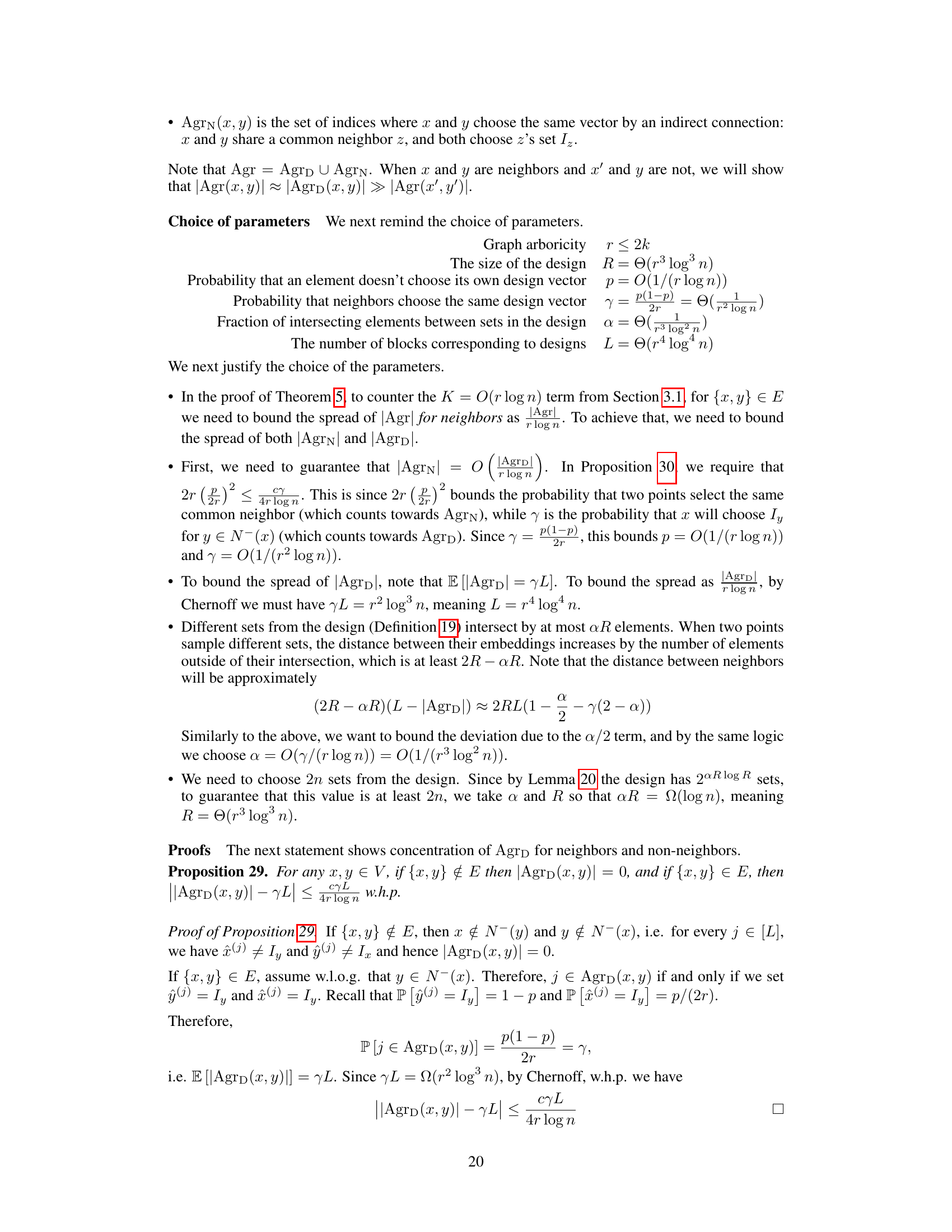
🔼 This table presents the training loss for preserving k-NNs (k-Nearest Neighbors) for different values of n (number of data points) and k (number of nearest neighbors considered). The loss measures how well the k-NN ordering is preserved in the learned embeddings. Lower values indicate better preservation of the k-NN structure. The table shows that the training loss increases with both n and k, indicating that preserving k-NN structure becomes more challenging as the number of data points and the number of neighbors to consider increase.
read the caption
Table 4: Training loss for preserving k-NNs for various values of n and k.
Full paper#
