TL;DR#
Point cloud analysis using masked point modeling (MPM) has seen significant improvements with Transformer-based models. However, these models suffer from quadratic complexity and limited decoder capabilities, hindering practical applications. The high computational cost and model size of these methods limit their use in resource-constrained settings. Existing Transformer-based MPM models also struggle to reconstruct masked patches with lower information density effectively.
To overcome these challenges, this paper presents LCM, a Locally Constrained Compact point cloud Model. LCM utilizes local aggregation layers to replace self-attention in the encoder, achieving linear complexity and significantly reducing parameters. A locally constrained Mamba-based decoder is used to efficiently handle varying information densities in the input. Extensive experiments demonstrate LCM’s superior performance and efficiency compared to Transformer-based models across various downstream tasks. This is achieved with a significant reduction in computational cost and model size.
Key Takeaways#
Why does it matter?#
This paper is crucial because it addresses the limitations of existing Transformer-based point cloud models, which are computationally expensive and have limited decoder capabilities. By introducing LCM, a more efficient and effective model, this research paves the way for broader applications of point cloud analysis in resource-constrained environments. It also offers a new perspective on information processing in point cloud modeling, prompting further research into more efficient and powerful architectures.
Visual Insights#
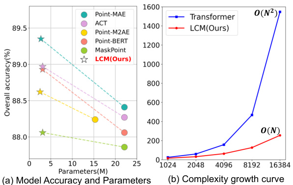
🔼 This figure compares the proposed LCM model with the traditional Transformer-based model in terms of accuracy and computational complexity. Subfigure (a) shows a comparison of the overall accuracy on ScanObjectNN against the number of model parameters (in millions). The LCM model achieves comparable accuracy with significantly fewer parameters than the Transformer model. Subfigure (b) illustrates the complexity growth curve as the input sequence length increases. The Transformer displays quadratic complexity (O(N²)), while the LCM demonstrates linear complexity (O(N)), highlighting its superior efficiency.
read the caption
Figure 1: Comparison of our LCM and Transformer in terms of performance and efficiency.
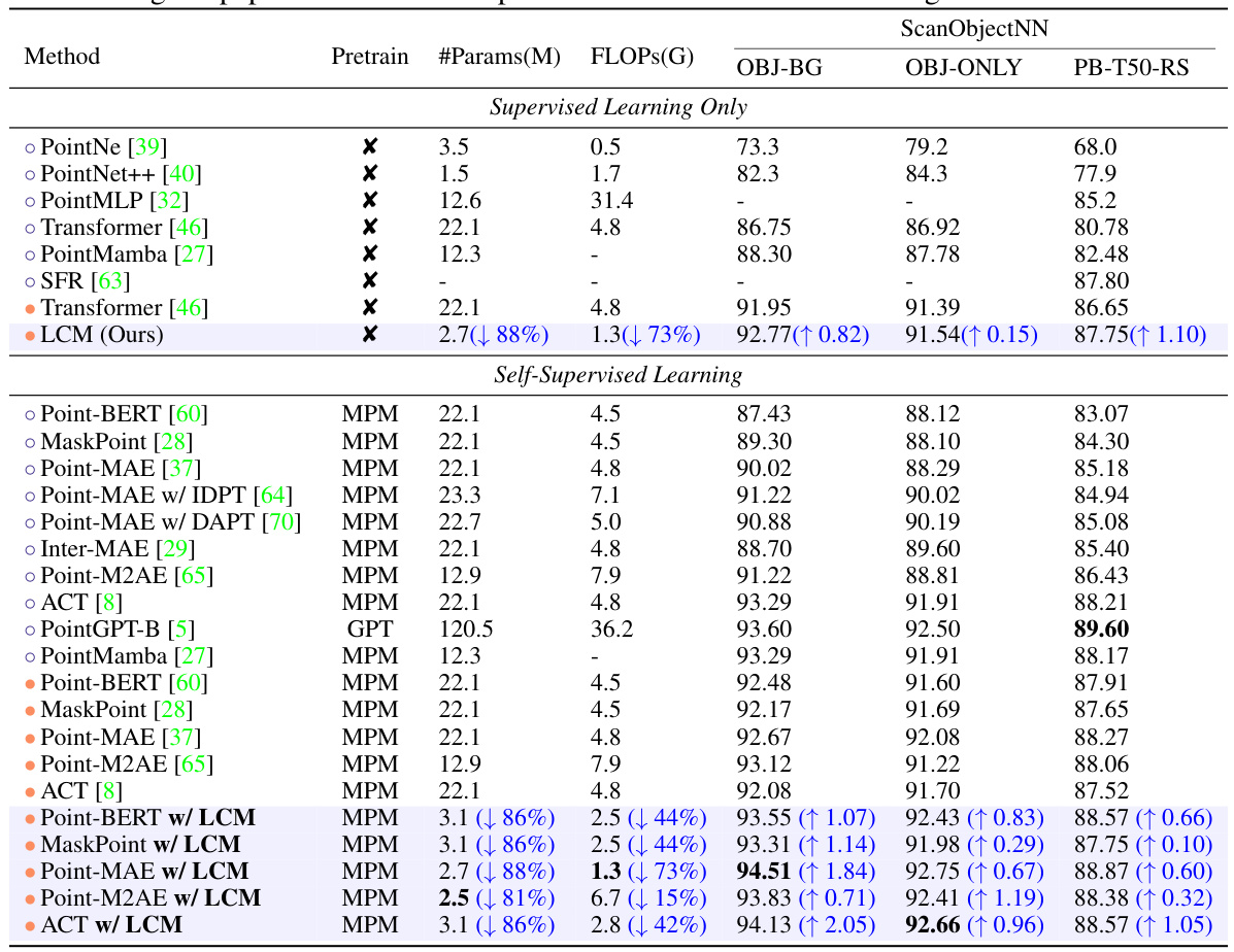
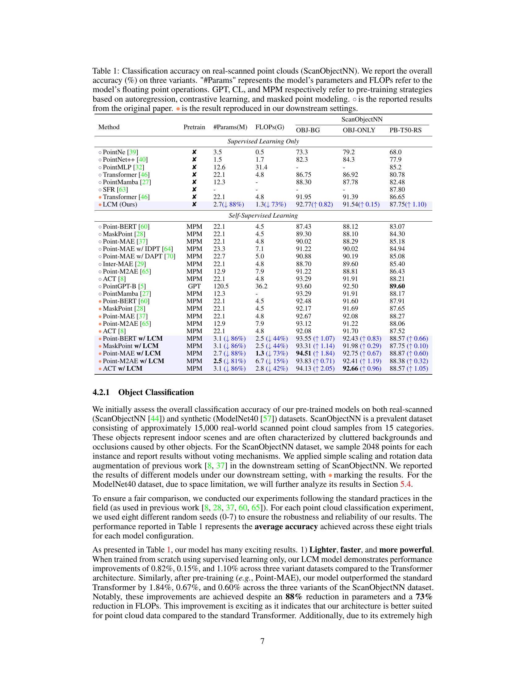
🔼 This table presents a comparison of various point cloud models on the ScanObjectNN dataset, focusing on classification accuracy. It includes both supervised and self-supervised learning methods, showcasing the performance of the proposed LCM model against existing state-of-the-art techniques. Key metrics such as model parameters (#Params), floating point operations (FLOPs), and classification accuracy on three different ScanObjectNN variants (OBJ-BG, OBJ-ONLY, PB-T50-RS) are presented, allowing for a comprehensive comparison of model efficiency and effectiveness.
read the caption
Table 1: Classification accuracy on real-scanned point clouds (ScanObjectNN). We report the overall accuracy (%) on three variants. '#Params' represents the model’s parameters and FLOPs refer to the model’s floating point operations. GPT, CL, and MPM respectively refer to pre-training strategies based on autoregression, contrastive learning, and masked point modeling. is the reported results from the original paper. is the result reproduced in our downstream settings.
In-depth insights#
LCM Architecture#
The LCM architecture, at its core, presents a novel approach to masked point cloud modeling that significantly departs from traditional Transformer-based methods. Its design prioritizes efficiency and effectiveness, replacing computationally expensive self-attention mechanisms with locally constrained operations. The compact encoder leverages local geometric constraints for aggregation, leading to linear time complexity and drastically reduced parameter count. The decoder employs a Mamba-based structure with LCFFN, enhancing the model’s ability to perceive higher-density unmasked patches while maintaining linear complexity and mitigating the order-dependency typically observed in vanilla SSM-based architectures. This combination of locally constrained encoding and decoding layers makes LCM exceptionally efficient while demonstrating superior performance, achieving a powerful balance between speed and accuracy for various point cloud tasks.
MPM Improvements#
Masked Point Modeling (MPM) has significantly advanced point cloud analysis, but existing Transformer-based MPM methods suffer from quadratic complexity and limited decoder capacity. This paper introduces key improvements to MPM by focusing on redundancy reduction. A novel locally constrained compact encoder replaces self-attention with efficient local aggregation, achieving a balance between performance and efficiency. Furthermore, a locally constrained Mamba-based decoder addresses the varying information density in MPM inputs by incorporating static local geometric constraints, maximizing information extraction from unmasked patches while maintaining linear complexity. The LCM-based Point-MAE model surpasses Transformer-based models in accuracy and efficiency, achieving considerable improvements on various benchmarks including ScanObjectNN, showcasing a clear advancement in masked point cloud modeling.
Ablation Studies#
Ablation studies systematically remove components of a model to assess their individual contributions. In this context, they would likely involve removing or modifying parts of the proposed LCM (Locally Constrained Compact Model) to understand the impact on performance. Key targets for ablation might include the local aggregation layers in the encoder, the locally constrained Mamba-based decoder, or the specific local constraint mechanisms used within these components. By observing the effects of these removals on downstream tasks like object classification or detection, researchers can determine the importance of each component to the overall model’s effectiveness. Results would reveal whether each module contributes significantly to performance improvements beyond a baseline, or if some parts are less crucial than others and could be removed to create a smaller, more efficient model. The ablation study should ideally also explore the influence of hyperparameter choices (such as the number of local aggregation layers) on the overall performance and efficiency tradeoff, providing a comprehensive understanding of the model’s design.
Future Work#
Future research directions stemming from this work could explore several promising avenues. Extending the LCM architecture to handle dynamic scenes and long-range dependencies is crucial for improving performance in complex environments. This might involve incorporating attention mechanisms or other methods to capture temporal information more effectively. Investigating alternative local aggregation strategies beyond the current KNN-based approach could yield significant improvements in both accuracy and efficiency. Exploring different types of local constraints, or developing more sophisticated methods for combining local and global information, are potential research areas. Developing more robust methods for handling noise and outliers is also critical, particularly in real-world point cloud data which is often noisy and incomplete. Analyzing the impact of different pre-training strategies on downstream tasks is another area warranting further investigation. Lastly, evaluating the LCM’s performance on larger, more diverse datasets, including those with a wider range of object categories and complexities, will be important for validating its generalizability and robustness.
Limitations#
A thoughtful analysis of the limitations section in a research paper is crucial for a comprehensive understanding. This section should explicitly address the shortcomings of the presented work, preventing any overselling of the results. It is important to acknowledge the scope of the research, for instance, a limited dataset size, constraints on computational resources, or the assumptions made that could influence results. Addressing the generalizability is also important; does the model’s performance hold true across different datasets, or is it restricted to a specific setting? Any methodological limitations should be described, such as the choice of specific algorithms or the potential impact of biases present in the data used. By acknowledging these limitations transparently, the research gains credibility and fosters trust, while also outlining future avenues for development and improvement. Finally, considering the broader impacts of the technology is paramount; are there any potential negative societal consequences that must be discussed? This in-depth perspective enhances the integrity and value of the study.
More visual insights#
More on figures

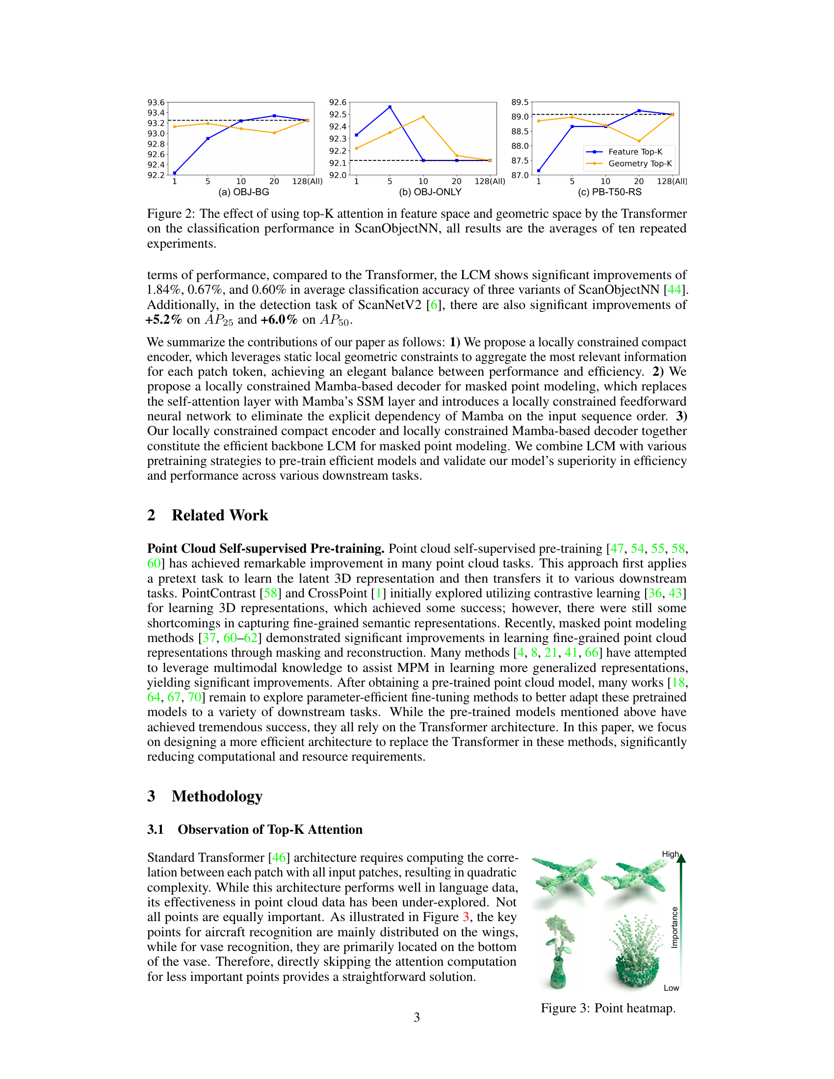
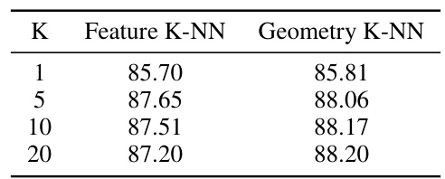
🔼 This figure shows the impact of using top-K attention on the classification performance in ScanObjectNN dataset. The experiment is conducted using different top-K values in both feature and geometric space, and the results are averaged over 10 repeated experiments. The results indicate that using top-K attention in a static geometric space yields nearly identical representational capacity and offers the advantage of a smaller K value, especially when compared with dynamic feature space.
read the caption
Figure 2: The effect of using top-K attention in feature space and geometric space by the Transformer on the classification performance in ScanObjectNN, all results are the averages of ten repeated experiments.

🔼 This figure shows heatmaps highlighting the importance of different points within point clouds representing an airplane and a vase. The color intensity indicates the importance of each point for object recognition, with darker green representing higher importance. For the airplane, the wings are highlighted as highly important, while for the vase, the base is the most important area. This visual representation helps illustrate the concept of varying information density across point clouds, highlighting that not all points carry equal significance for object recognition tasks, a crucial observation that underpins the design of the Locally Constrained Compact Model (LCM).
read the caption
Figure 3: Point heatmap.

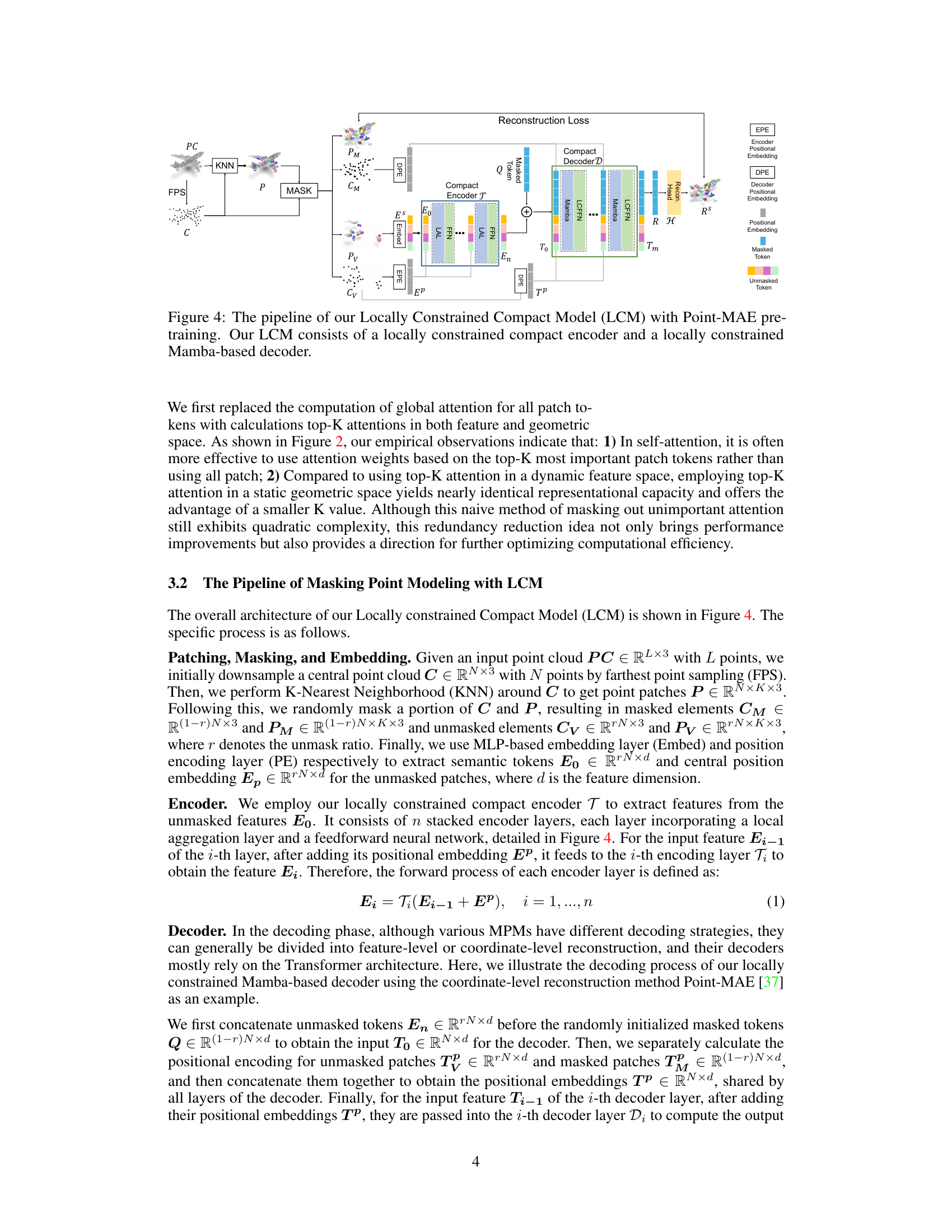
🔼 This figure illustrates the architecture of the Locally Constrained Compact Model (LCM) for masked point modeling. The LCM comprises two main parts: a locally constrained compact encoder and a locally constrained Mamba-based decoder. The encoder takes unmasked point cloud patches as input and uses local aggregation layers instead of self-attention to reduce computational complexity. The decoder receives both unmasked and masked tokens, utilizing a Mamba-based architecture to reconstruct the masked tokens by leveraging the information density differences between masked and unmasked patches and incorporating local geometric constraints. The overall process involves patching, masking, embedding, encoding, decoding, and finally reconstruction based on a reconstruction loss function.
read the caption
Figure 4: The pipeline of our Locally Constrained Compact Model (LCM) with Point-MAE pre-training. Our LCM consists of a locally constrained compact encoder and a locally constrained Mamba-based decoder.

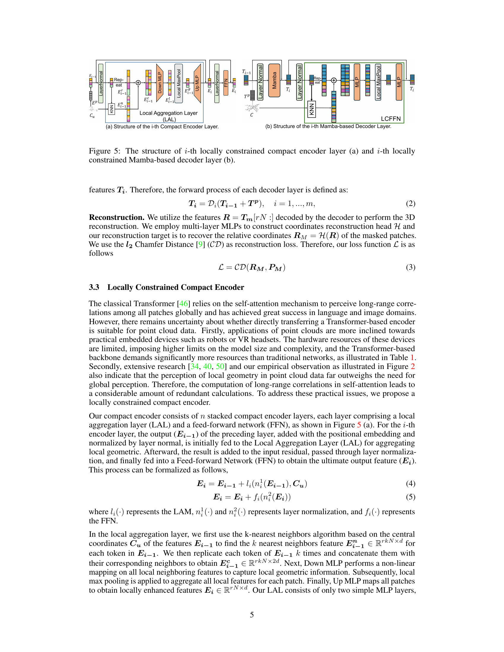
🔼 This figure shows the detailed architecture of the i-th layer of both the encoder and decoder used in the LCM model. The encoder layer (a) consists of a local aggregation layer (LAL) incorporating KNN for local geometric information gathering, followed by MLPs for feature mapping and a feed-forward network (FFN). The decoder layer (b) combines a Mamba-based SSM layer for capturing temporal dependencies and a local constraints feedforward network (LCFFN) to exchange information among geometrically adjacent patches, effectively improving the accuracy while minimizing computation cost.
read the caption
Figure 5: The structure of i-th locally constrained compact encoder layer (a) and i-th locally constrained Mamba-based decoder layer (b).
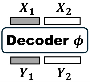
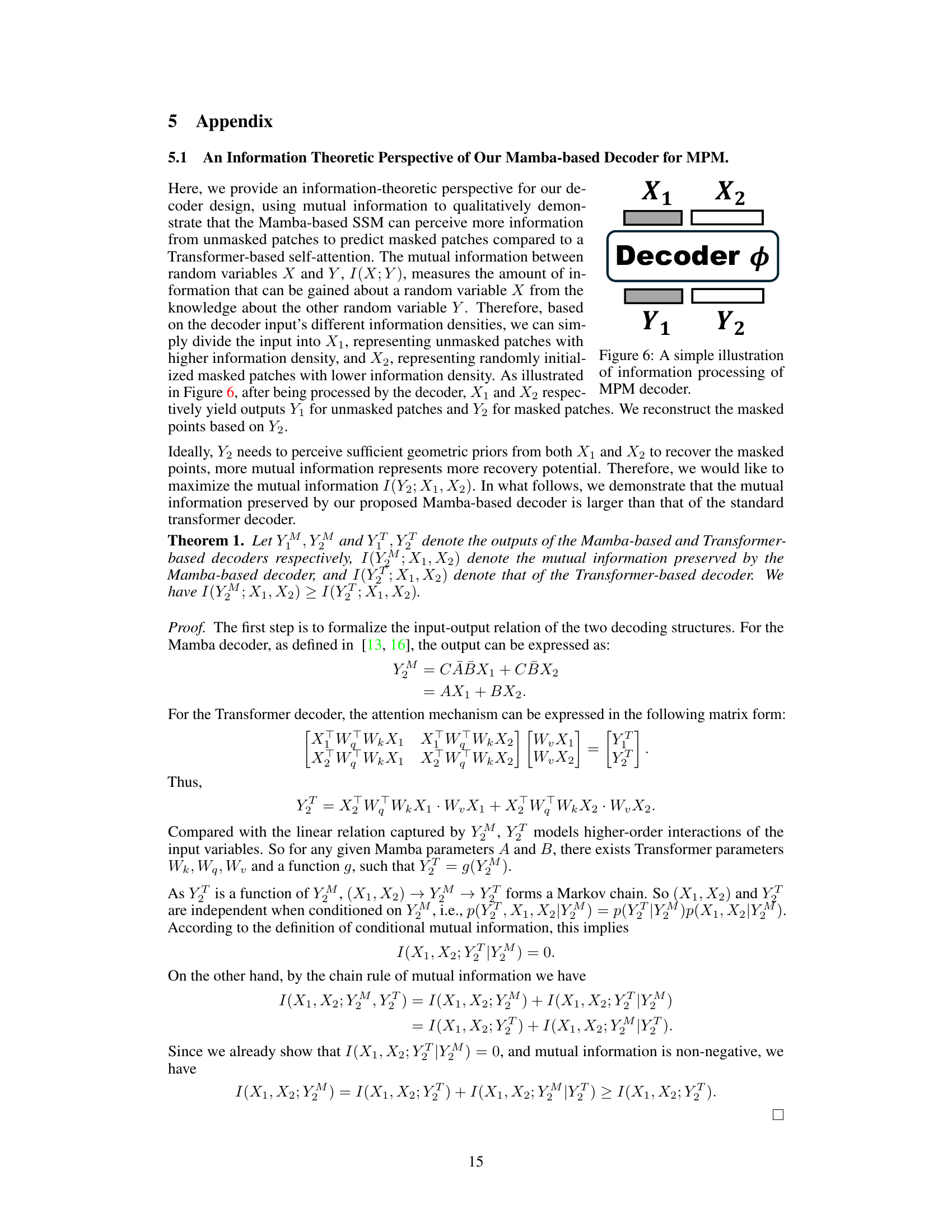
🔼 This figure illustrates the information processing in the decoder of a masked point modeling (MPM) model. The input consists of two parts: X1 (unmasked patches with higher information density) and X2 (randomly initialized masked patches with lower information density). The decoder processes these inputs, producing outputs Y1 (for unmasked patches) and Y2 (for masked patches). The goal is to reconstruct the masked points (X2) using the information from Y2, which ideally should utilize geometric priors from both X1 and X2. The figure visually represents the flow of information through the decoder.
read the caption
Figure 6: A simple illustration of information processing of MPM decoder.
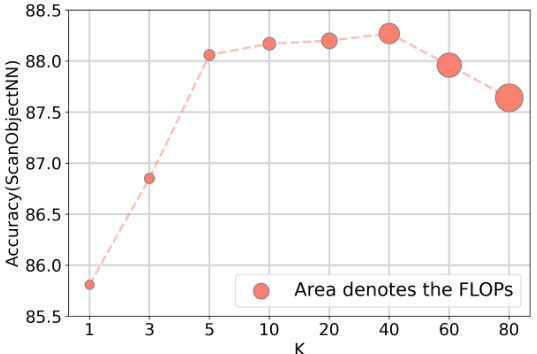
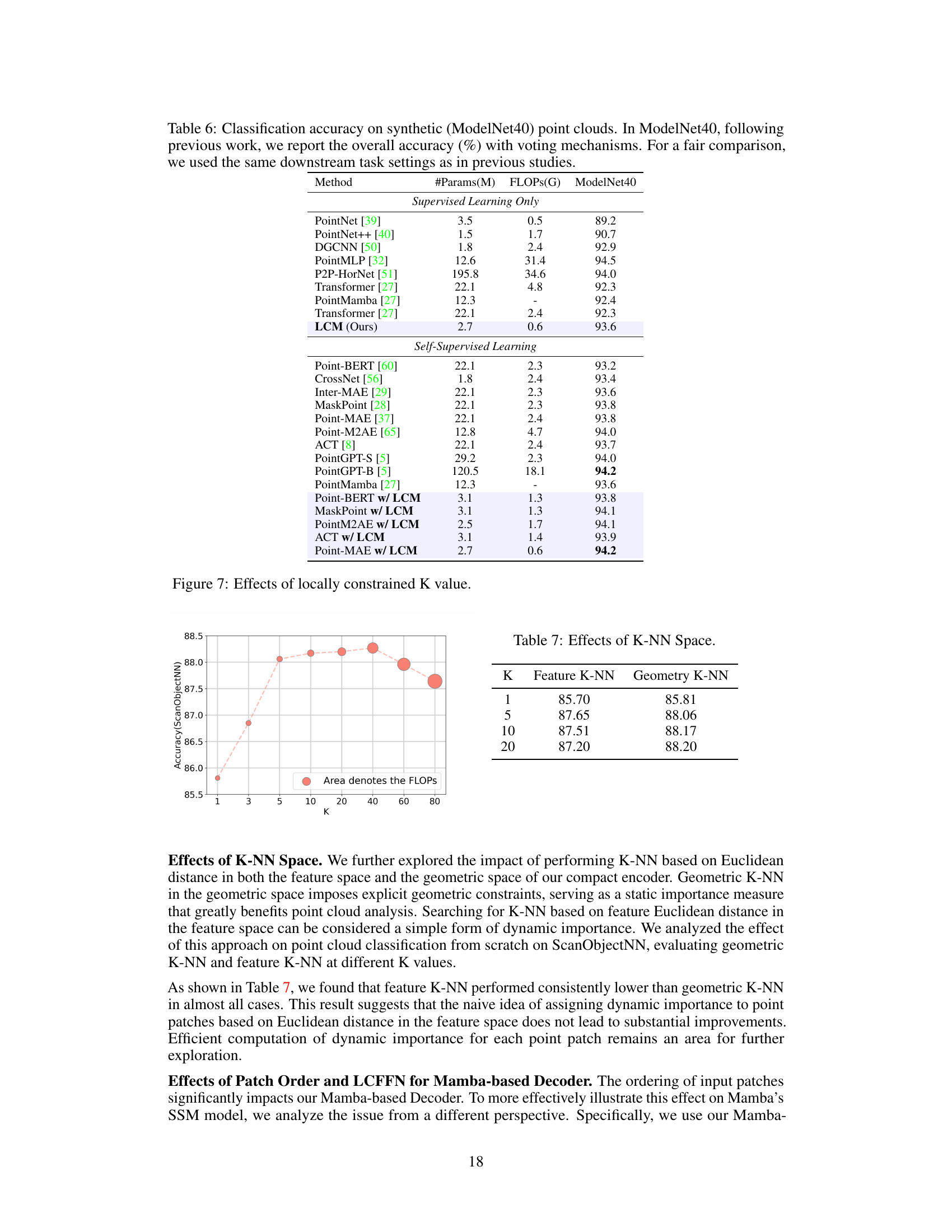
🔼 This figure shows the relationship between the number of nearest neighbors (K) used in local aggregation and the classification accuracy on the ScanObjectNN dataset. As K increases, the model considers more neighbors, potentially capturing more local geometric information, leading to increased accuracy initially. However, after reaching a peak, further increasing K leads to reduced accuracy, likely due to the introduction of redundant or less relevant information from distant neighbors. The area of the circles represents the FLOPS (floating point operations), indicating the computational cost associated with each K value.
read the caption
Figure 7: Effects of locally constrained K value.

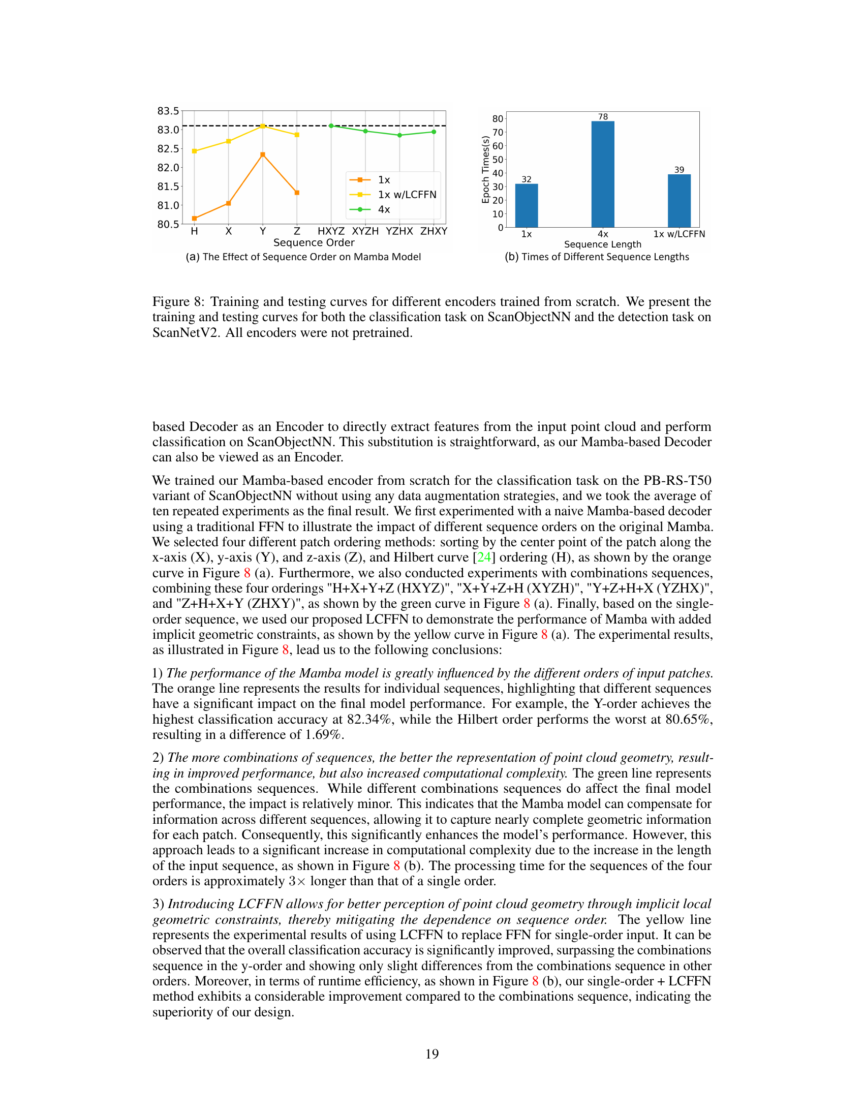
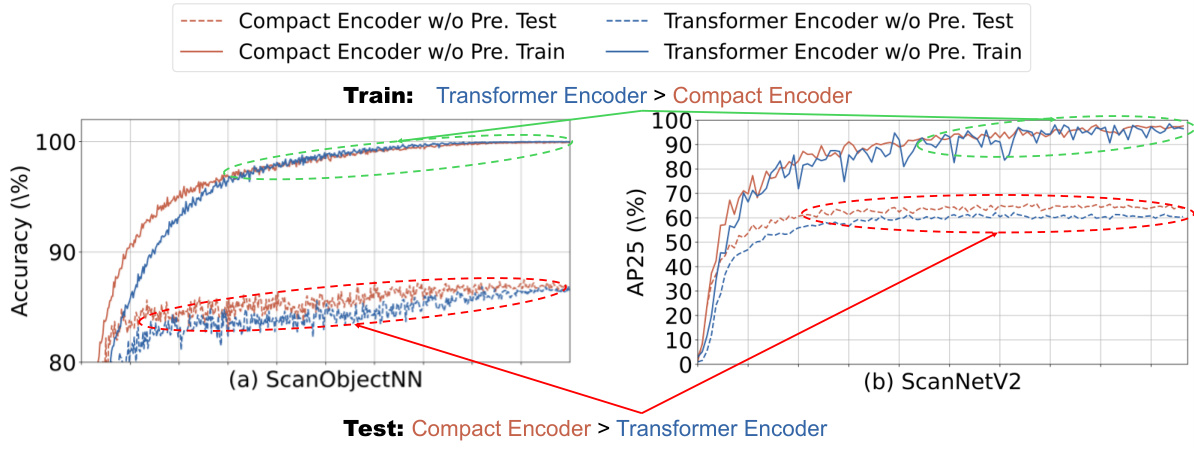
🔼 This figure compares the training and testing curves of different encoders (Mamba with and without LCFFN, and 4x Mamba) for classification (ScanObjectNN) and detection (ScanNetV2) tasks. The results show that the order of the input sequences significantly affects the Mamba-based model’s performance, while the addition of LCFFN mitigates this order dependence and improves efficiency. The figure highlights the trade-off between model performance and computational cost associated with different sequence ordering strategies.
read the caption
Figure 8: Training and testing curves for different encoders trained from scratch. We present the training and testing curves for both the classification task on ScanObjectNN and the detection task on ScanNetV2. All encoders were not pretrained.
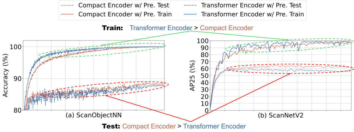
🔼 This figure compares the training and testing curves of a compact encoder and a transformer encoder, both pre-trained. The results show that while the transformer encoder achieves higher accuracy during training, the compact encoder exhibits superior performance during testing, indicating better generalization and less overfitting.
read the caption
Figure 9: Training and testing curves of different pre-trained encoders. We present the training and testing curves for both the classification task on ScanObjectNN and the detection task on ScanNetV2. All encoders are pre-trained.
🔼 This figure shows a comparison of the training and testing curves for a compact encoder and a transformer encoder, both pre-trained on the same dataset. The left plot displays the classification accuracy on the ScanObjectNN dataset, while the right plot shows the average precision at 25% Intersection over Union (AP25) on the ScanNetV2 dataset. The results indicate that while the transformer encoder performs better during training, suggesting a potential overfitting to the training data, the compact encoder achieves superior performance during testing, highlighting its better generalization ability.
read the caption
Figure 9: Training and testing curves of different pre-trained encoders. We present the training and testing curves for both the classification task on ScanObjectNN and the detection task on ScanNetV2. All encoders are pre-trained.
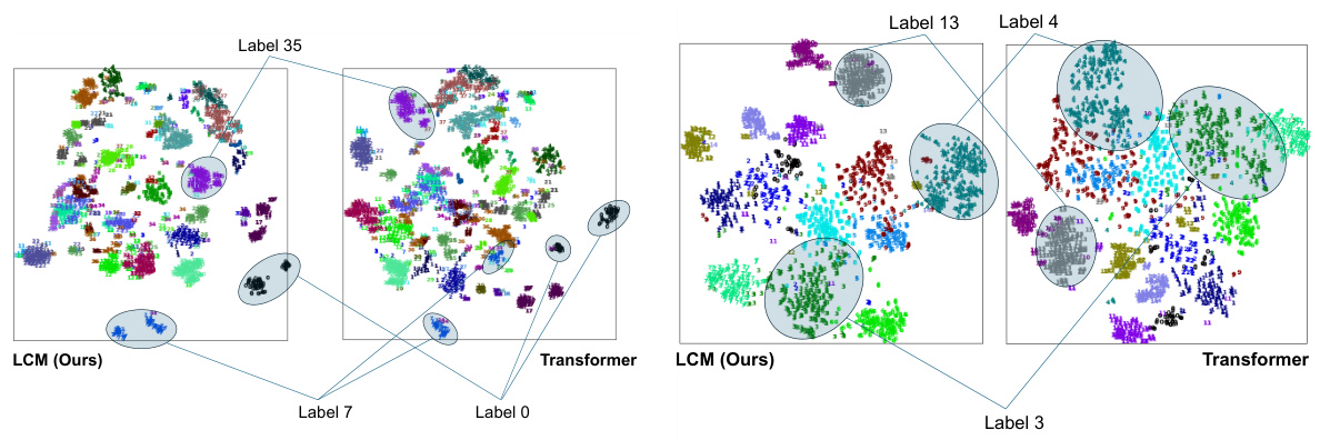
🔼 This figure visualizes the feature distributions extracted by the LCM and Transformer models pretrained using Point-MAE, directly transferred to the test set of ModelNet40 without downstream finetuning. It uses t-SNE to reduce the dimensionality of the features to 2D for visualization. Each dot represents an instance from ModelNet40, and the color indicates its category. The compactness of the clusters shows the model’s ability to represent features of the same category.
read the caption
Figure 11: The feature distribution visualization of the pre-trained models on the test set of ModelNet40.
More on tables
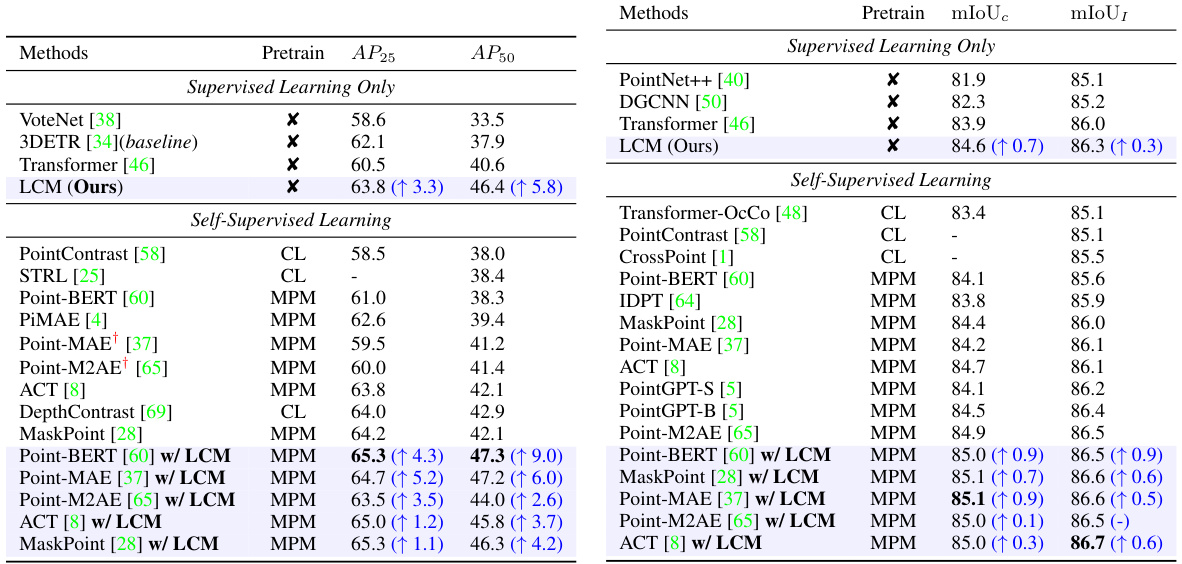
🔼 This table presents a comparison of various point cloud models’ performance on the ScanObjectNN dataset, focusing on classification accuracy. It breaks down the results by pre-training method (autoregressive, contrastive learning, masked point modeling), showing the overall accuracy, number of parameters, and floating point operations for each model. The table also includes comparisons to results reported in original papers and results reproduced by the authors using consistent downstream settings. This allows for a comprehensive assessment of model efficiency and accuracy.
read the caption
Table 1: Classification accuracy on real-scanned point clouds (ScanObjectNN). We report the overall accuracy (%) on three variants. '#Params' represents the model's parameters and FLOPs refer to the model's floating point operations. GPT, CL, and MPM respectively refer to pre-training strategies based on autoregression, contrastive learning, and masked point modeling. is the reported results from the original paper. is the result reproduced in our downstream settings.

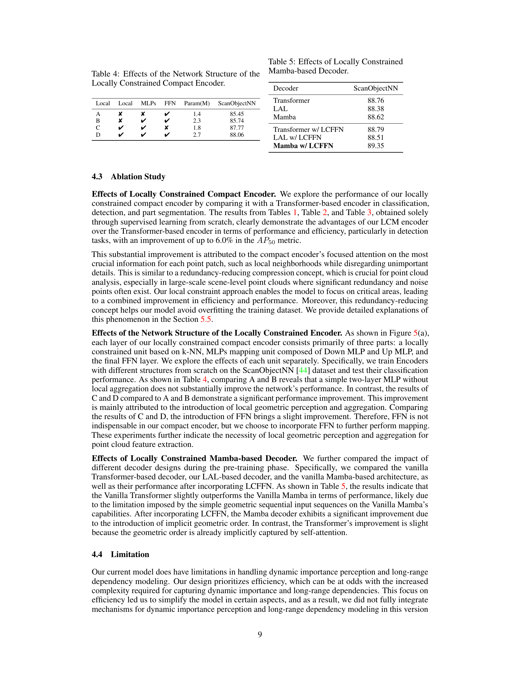
🔼 This table presents an ablation study on the locally constrained compact encoder, showing the impact of different components (Local Aggregation Layer, MLPs, FFN) on the model’s performance (ScanObjectNN accuracy). It demonstrates the importance of local geometric perception and aggregation for point cloud feature extraction. Comparing the results of configurations A through D indicates that including a local aggregation layer and MLPs significantly improves performance, while the FFN provides a small additional benefit.
read the caption
Table 4: Effects of the Network Structure of the Locally Constrained Compact Encoder.
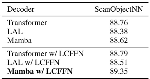
🔼 This table presents the ablation study results, focusing on the impact of different decoder architectures on the performance of the model. It compares the performance of a standard Transformer decoder against a locally constrained Mamba-based decoder, both with and without the addition of a Local Constraints Feedforward Network (LCFFN). The results are shown in terms of classification accuracy on the ScanObjectNN dataset.
read the caption
Table 5: Effects of Locally Constrained Mamba-based Decoder.
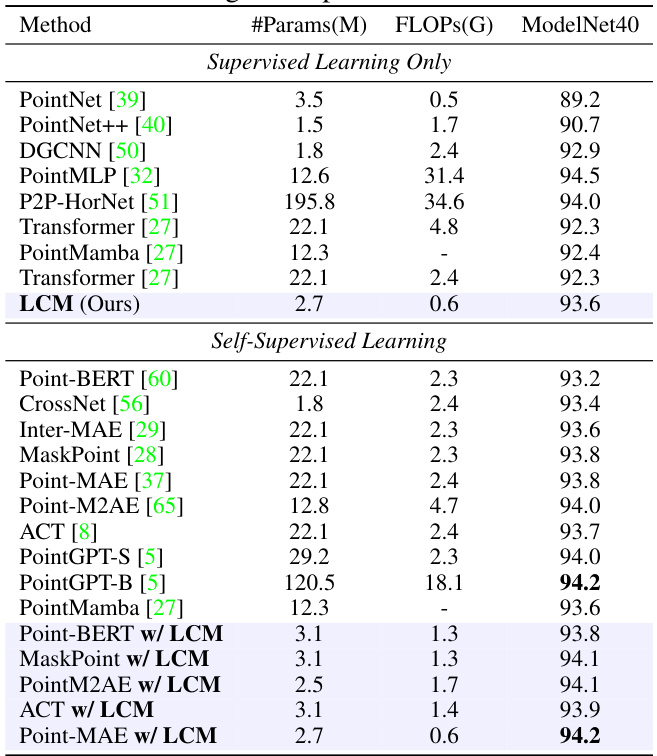
🔼 This table presents a comparison of various point cloud models’ performance on the ScanObjectNN dataset, focusing on classification accuracy. It breaks down the results by different pre-training methods (GPT, CL, MPM), showing overall accuracy, the number of parameters (#Params), and floating point operations (FLOPs). The table also highlights the improvements achieved by the proposed LCM model compared to existing Transformer-based models. Both original reported and reproduced results are included.
read the caption
Table 1: Classification accuracy on real-scanned point clouds (ScanObjectNN). We report the overall accuracy (%) on three variants. '#Params' represents the model’s parameters and FLOPs refer to the model’s floating point operations. GPT, CL, and MPM respectively refer to pre-training strategies based on autoregression, contrastive learning, and masked point modeling. is the reported results from the original paper. is the result reproduced in our downstream settings.
🔼 This table compares the performance of various point cloud models on the ScanObjectNN dataset, focusing on classification accuracy. It breaks down the results by three variants of the dataset and includes the number of parameters (#Params), floating point operations (FLOPs), and pre-training strategy used for each model (GPT, CL, MPM). It also notes whether results are from the original papers or reproduced by the authors. The table highlights the performance improvements achieved by LCM compared to other models.
read the caption
Table 1: Classification accuracy on real-scanned point clouds (ScanObjectNN). We report the overall accuracy (%) on three variants. '#Params' represents the model's parameters and FLOPs refer to the model's floating point operations. GPT, CL, and MPM respectively refer to pre-training strategies based on autoregression, contrastive learning, and masked point modeling. is the reported results from the original paper. is the result reproduced in our downstream settings.
Full paper#
