↗ OpenReview ↗ NeurIPS Homepage ↗ Chat
TL;DR#
3D medical image reconstruction, such as in Computed Tomography (CT), faces challenges due to high dimensionality and data demands. Existing diffusion-based methods often struggle with this, using 2D slices and hand-crafted regularization, resulting in artifacts and z-axis inconsistencies. This limits their ability to accurately learn a comprehensive 3D image prior for accurate reconstruction.
DiffusionBlend++, a novel approach, learns the 3D image prior through position-aware 3D-patch diffusion score blending. This innovative technique combines information from neighboring 2D slices in 3D patches and blends their scores, overcoming the inconsistencies of previous methods. Extensive experiments on sparse-view and limited-angle CT show that DiffusionBlend++ significantly outperforms previous methods, leading to state-of-the-art performance. It is computationally efficient and requires minimal hyperparameter tuning.
Key Takeaways#
Why does it matter?#
This paper is significant as it presents a novel approach to 3D medical image reconstruction using 3D diffusion priors, overcoming the limitations of existing methods. This advance could significantly improve the quality and efficiency of medical imaging, leading to better diagnoses and treatments. The methodology is also relevant to broader inverse problems and inspires new avenues for research in high-dimensional data processing.
Visual Insights#
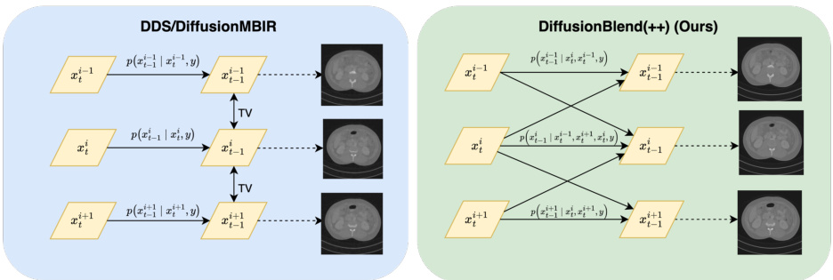
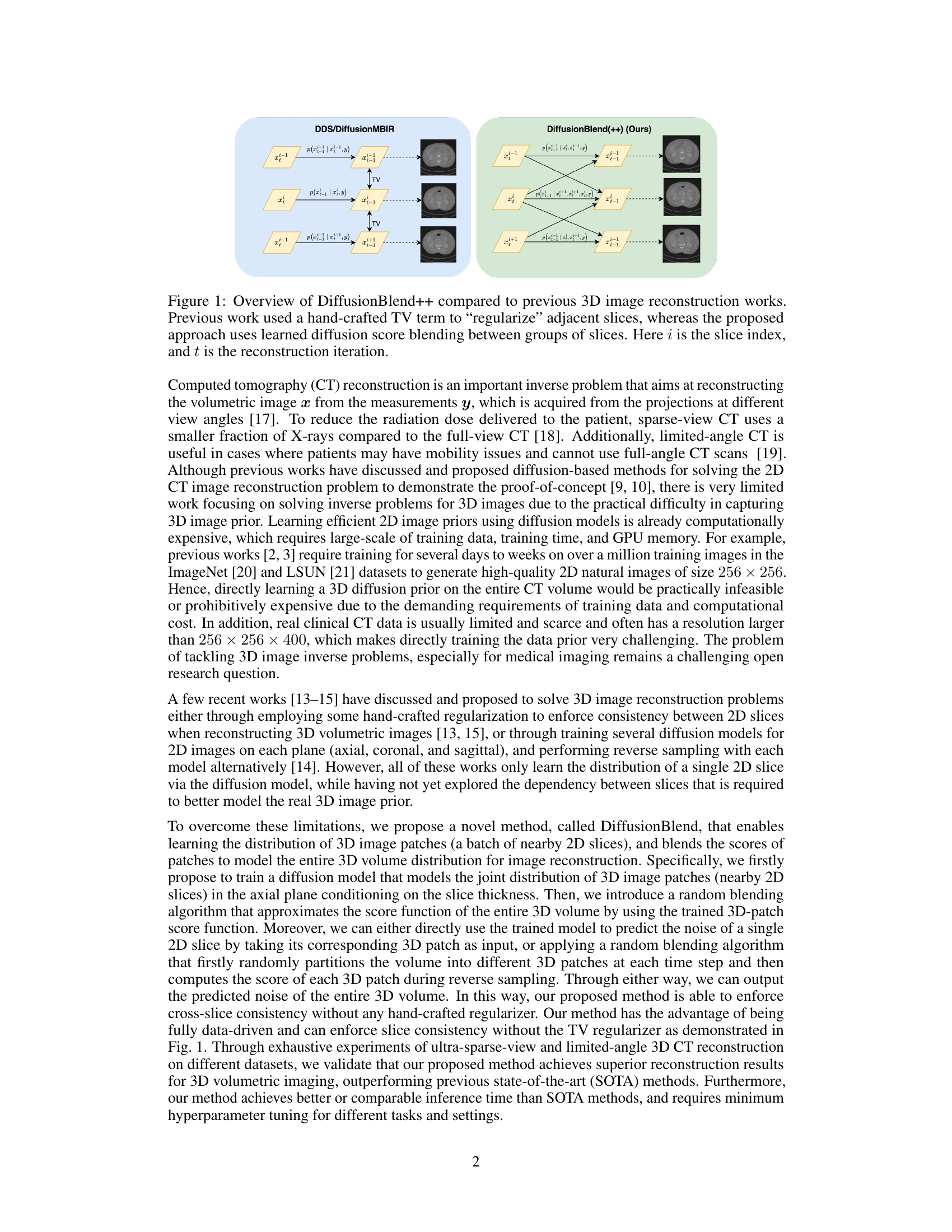
This figure compares the proposed DiffusionBlend++ method with previous 3D image reconstruction methods. Previous methods used a hand-crafted total variation (TV) term to regularize adjacent slices, resulting in a loss of z-axis consistency. DiffusionBlend++, on the other hand, uses a learned diffusion score blending method between groups of slices, improving z-axis consistency and reducing artifacts.

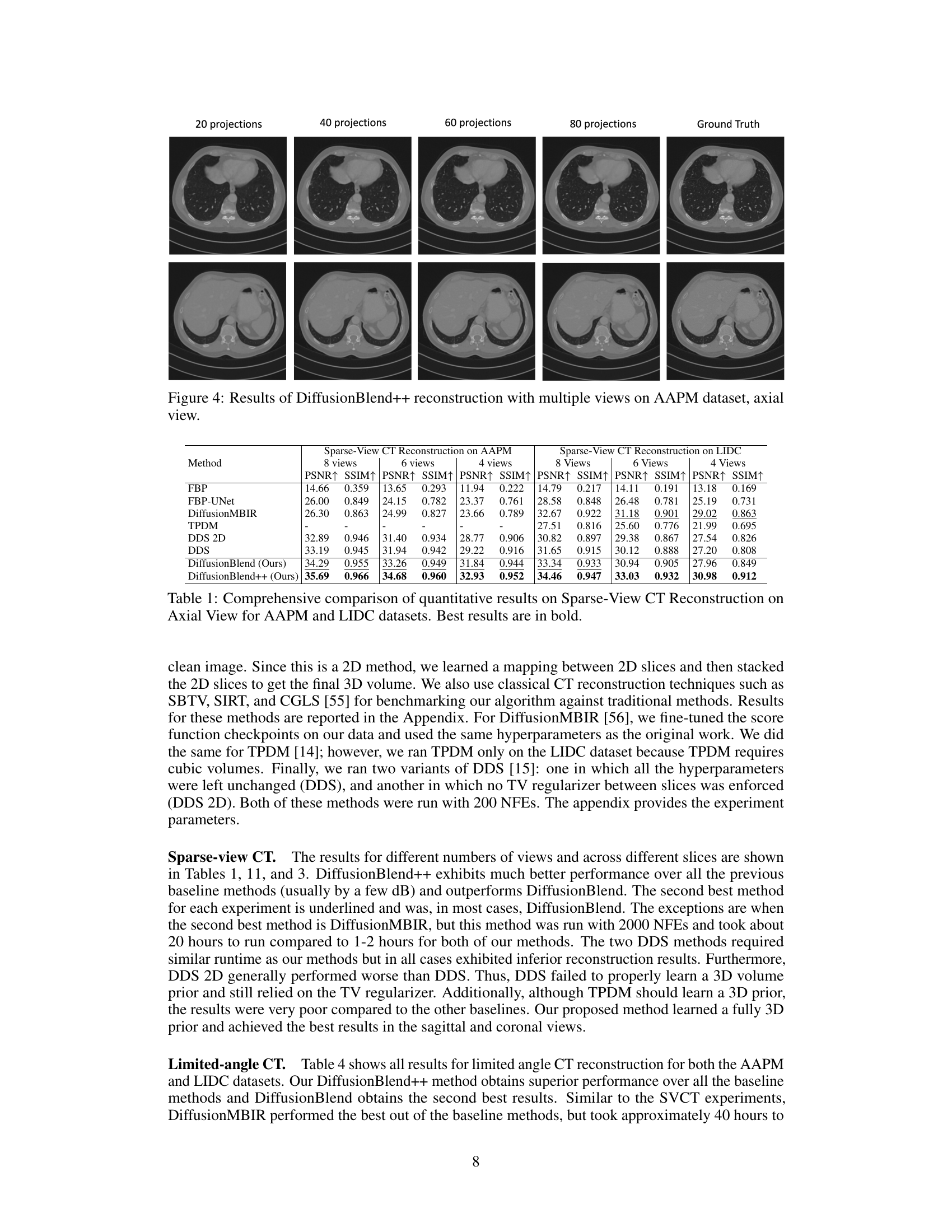
This table presents a quantitative comparison of different methods for sparse-view computed tomography (CT) reconstruction. The metrics used for comparison are PSNR (Peak Signal-to-Noise Ratio) and SSIM (Structural Similarity Index). Results are shown for both the AAPM and LIDC datasets (two different CT datasets), and for varying numbers of views (8, 6, and 4). The best performing method for each metric and dataset is highlighted in bold. The table helps readers quickly assess the relative performance of the different CT reconstruction algorithms.
In-depth insights#
3D Diffusion Prior#
The concept of a ‘3D Diffusion Prior’ in medical image reconstruction represents a significant advancement, addressing the limitations of existing 2D approaches. Directly applying diffusion models to entire 3D volumes is computationally expensive and memory-intensive. The challenge lies in learning a meaningful 3D image prior that captures the intricate relationships between slices without sacrificing efficiency. Therefore, innovative strategies such as employing 3D image patches, or cleverly blending diffusion scores from multiple 2D slices, become crucial for creating a powerful yet practical 3D diffusion prior. The effectiveness of such strategies hinges on successfully capturing cross-slice dependencies and ensuring computational feasibility. By learning from 3D patches, the model can implicitly learn this dependency, leading to improved reconstruction accuracy and reducing artifacts compared to handcrafted regularization methods. This leads to superior reconstruction results, particularly in challenging scenarios like sparse-view and limited-angle computed tomography. The development of computationally efficient algorithms for handling the high dimensionality of 3D data is key to the success of this methodology.
Score Function Blend#
The concept of ‘Score Function Blend’ in the context of diffusion models for 3D image reconstruction presents a compelling approach to address the limitations of existing methods. By blending the score functions of multiple 2D slices or 3D patches, this technique aims to learn a more comprehensive and consistent 3D image prior. This contrasts with methods that treat slices independently, which can lead to inconsistencies along the z-axis. A key advantage is its ability to incorporate cross-slice dependencies without relying on hand-crafted regularizers, leading to potentially better reconstruction quality. The success of this approach hinges on the effectiveness of the blending algorithm and the training methodology used to learn the score functions. A crucial aspect is the proper handling of boundary conditions and the balance between computational efficiency and model accuracy. Thorough experimentation on diverse datasets and comparison against state-of-the-art methods are essential to validate the efficacy and robustness of ‘Score Function Blend’ for various 3D image reconstruction tasks.
CT Reconstruction#
The research paper explores 3D computed tomography (CT) reconstruction, a crucial inverse problem in medical imaging. The core challenge lies in efficiently learning a 3D image prior from limited data and high dimensionality. The paper proposes a novel framework, DiffusionBlend, that utilizes 3D-patch diffusion score blending to effectively capture cross-slice dependencies, improving the accuracy and consistency of 3D CT reconstructions compared to existing 2D-slice methods. The use of position-aware 3D patches is key, as it enables learning the 3D image prior directly. This approach outperforms prior methods that rely on hand-crafted regularizations or learning independent priors for each 2D slice. DiffusionBlend demonstrates state-of-the-art performance on real-world CT datasets, while offering improved computational efficiency.
DiffusionBlend++#
DiffusionBlend++, as a novel method, significantly enhances 3D medical image reconstruction by leveraging 3D diffusion priors. Unlike previous methods that process individual 2D slices, DiffusionBlend++ cleverly blends scores from 3D image patches, capturing crucial cross-slice dependencies and thus improving z-axis consistency. This approach enables learning of a more realistic 3D image prior leading to superior reconstruction quality, especially in challenging scenarios like sparse-view or limited-angle CT scans. The method’s effectiveness is validated through extensive experiments showcasing state-of-the-art performance and competitive efficiency. Furthermore, the incorporation of positional encoding refines the model’s ability to handle non-adjacent slices, contributing to enhanced reconstruction accuracy and robustness. The random blending strategy employed during reconstruction adds to the method’s flexibility and computational efficiency. Overall, DiffusionBlend++ presents a substantial advancement in 3D image reconstruction, offering a more comprehensive and effective approach.
Future Research#
Future research directions stemming from this work on 3D CT reconstruction using diffusion models could explore several promising avenues. Improving computational efficiency remains a key challenge; investigating alternative network architectures or training strategies could significantly reduce processing times. The approach’s robustness to noisy real-world data should be thoroughly evaluated, potentially through incorporating techniques for handling uncertainties and artifacts. Furthermore, extending the methodology to other imaging modalities such as MRI or ultrasound would demonstrate wider applicability and impact. Finally, exploring the use of generative models beyond reconstruction, perhaps for image synthesis or data augmentation, opens intriguing possibilities for enhancing medical image analysis and diagnosis. This could include exploring different types of diffusion models or hybrid approaches that combine deep learning with physics-based priors.
More visual insights#
More on figures
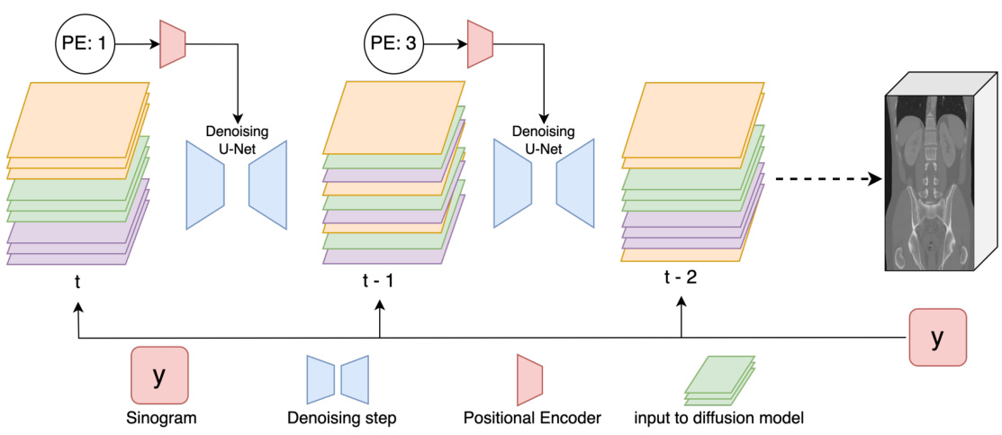
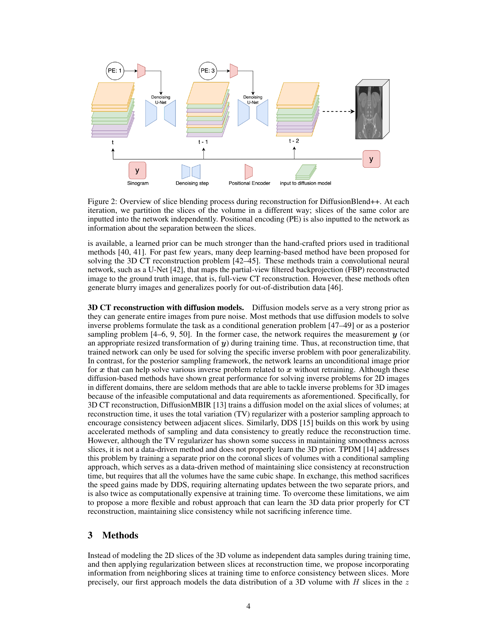
This figure illustrates the slice blending process within the DiffusionBlend++ algorithm during 3D image reconstruction. At each iteration (time step t, t-1, t-2), the volume’s slices are divided into groups (same color). Each group is processed independently by a denoising U-Net, incorporating positional encoding (PE) to account for slice separation. This positional encoding provides information on the spatial arrangement of the slices in the 3D volume. The sinogram (measurement data, y) is inputted to the process and provides contextual information. The process iteratively refines the reconstruction from noisy initial conditions, gradually reducing noise in multiple steps until a final 3D volume is produced.

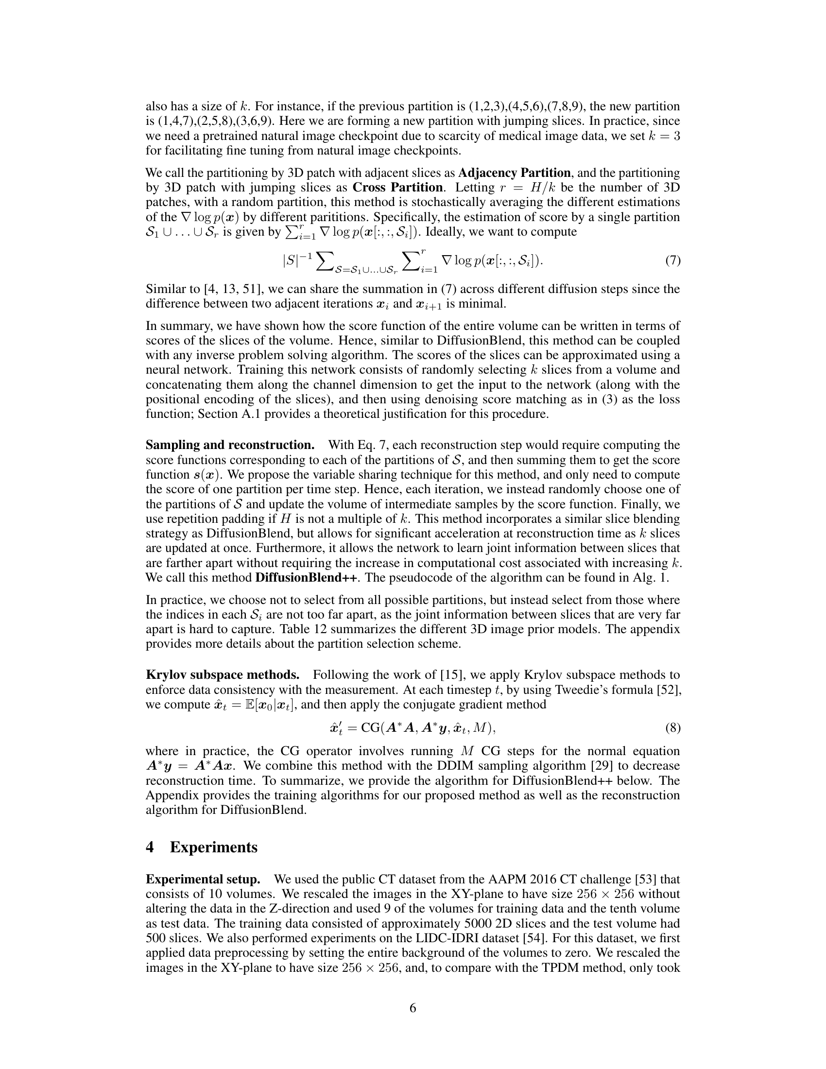
This figure shows a visual comparison of the results of CT reconstruction using 4 views on the AAPM dataset, focusing on the axial view. It compares the performance of several methods: Filtered Back Projection (FBP), FBP-UNet, DDS, DDS 2D, the proposed method (Ours), and the ground truth. The red boxes highlight regions of interest where the different methods’ performance can be visually assessed. The figure demonstrates the superior quality of the proposed method compared to the others in reconstructing fine details and overall image fidelity.
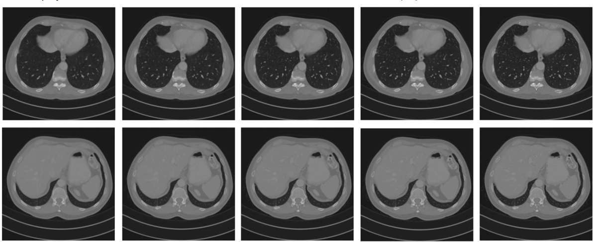
This figure shows the results of computed tomography (CT) reconstruction using 4 views of the AAPM dataset. It compares the performance of different reconstruction methods, including FBP, FBP-UNet, DDS, DDS 2D, and DiffusionBlend++. The axial view of the reconstructed images is shown. The ground truth image is also included for comparison.
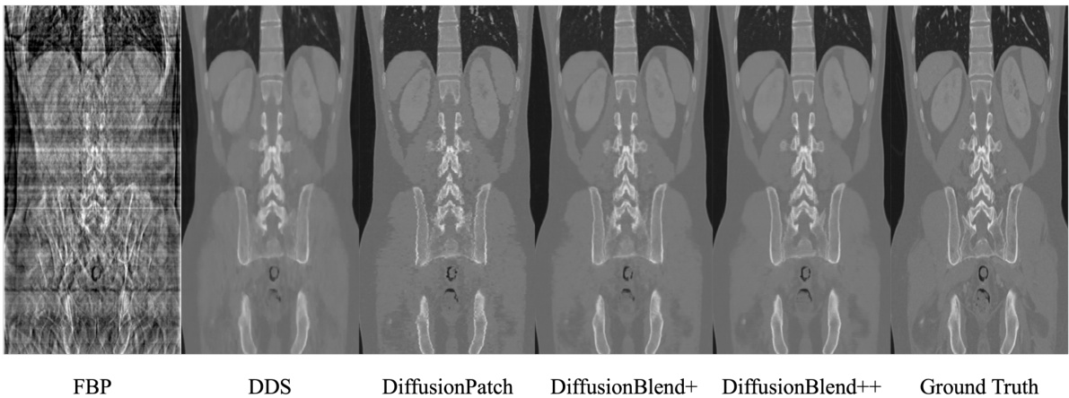
This figure compares the results of CT reconstruction using different methods (FBP, FBP-UNet, DDS, DDS 2D, and the proposed DiffusionBlend++) with 4 views on the AAPM dataset. The axial view of the reconstructed CT images is shown for each method. It demonstrates the superior performance of the proposed method compared to the baselines, particularly in terms of image quality and artifact reduction.

This figure shows the results of computed tomography (CT) reconstruction using 4 views on the AAPM dataset. The axial view is displayed. The figure compares the reconstruction quality of several methods including FBP, FBP-UNet, DDS, DDS 2D, and the proposed DiffusionBlend++ method. The ground truth image is also shown for comparison.

This figure compares the axial view of CT reconstruction results using different methods on the AAPM dataset with only 4 views. It shows that DiffusionBlend++ produces a significantly more accurate reconstruction compared to other methods, including Filtered Back Projection (FBP), FBP-UNet, DDS, and DDS 2D. The ground truth image is also shown for comparison. The improved quality highlights the effectiveness of the DiffusionBlend++ approach in reconstructing high-dimensional 3D images from limited data.

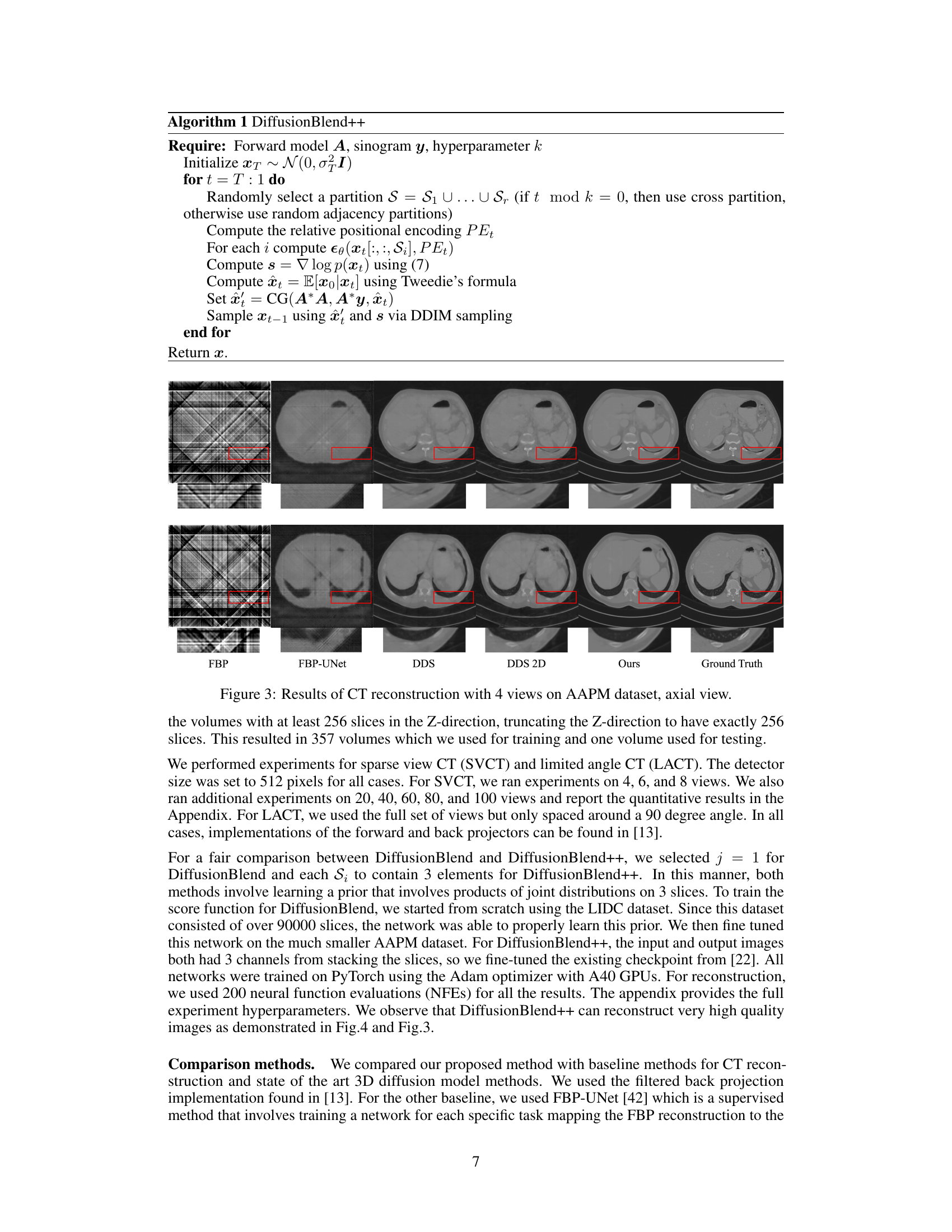
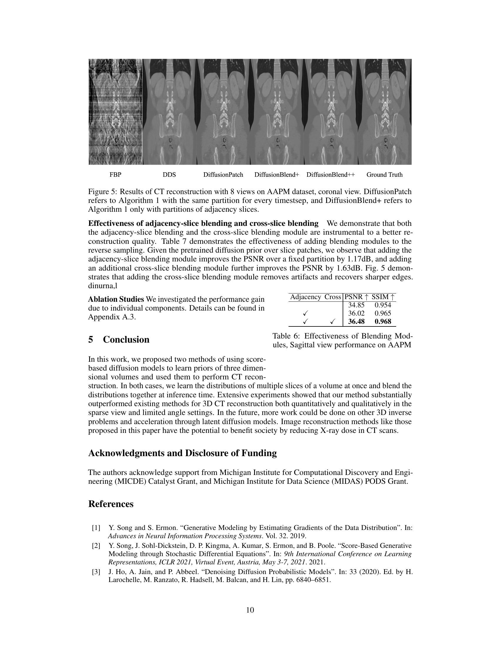
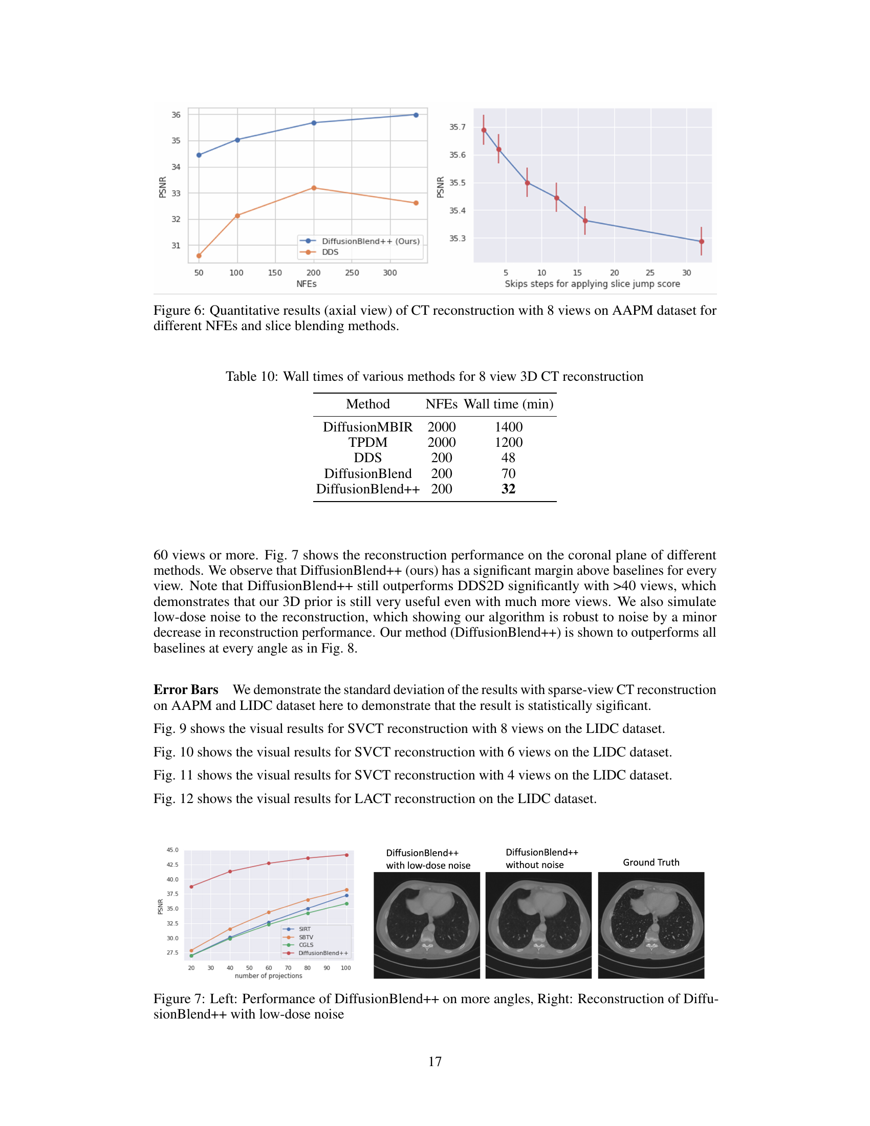
This figure compares the results of CT reconstruction using DiffusionBlend++ against three classical methods: SBTV, SIRT, and DDS. Each method’s reconstruction is shown alongside the ground truth image. The purpose is to visually demonstrate the superior performance of DiffusionBlend++ in terms of image quality and detail preservation compared to these traditional techniques.
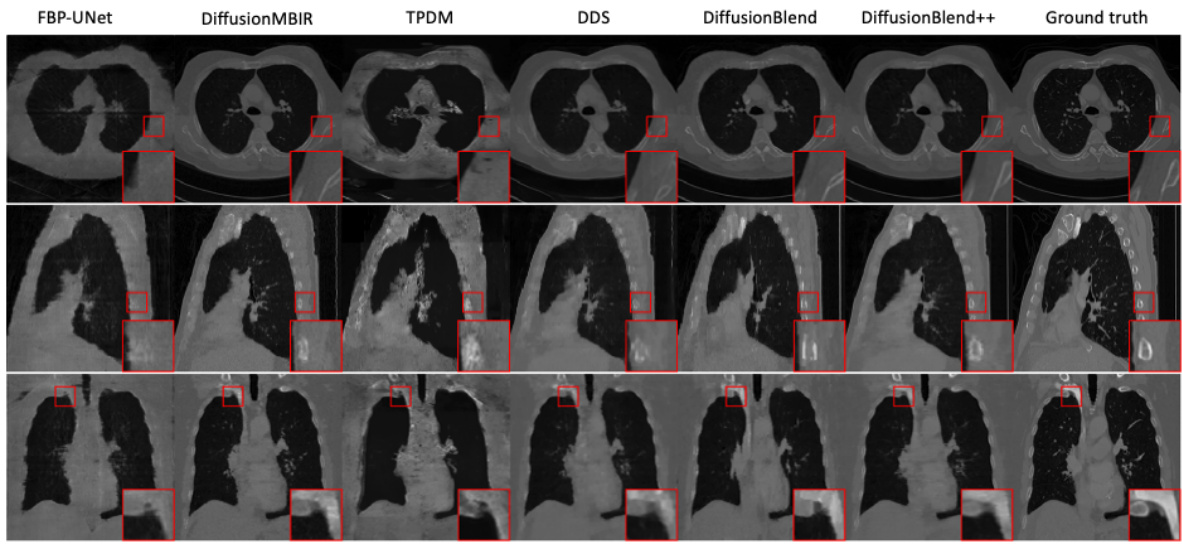
This figure compares the results of CT reconstruction using different methods (FBP, FBP-UNet, DDS, DDS 2D, and DiffusionBlend++) with 4 views on the AAPM dataset. The axial view of the reconstructed volume is shown for each method. The ground truth is also included for comparison. It visually demonstrates the superior performance of DiffusionBlend++ in terms of image quality and detail preservation compared to the other methods.
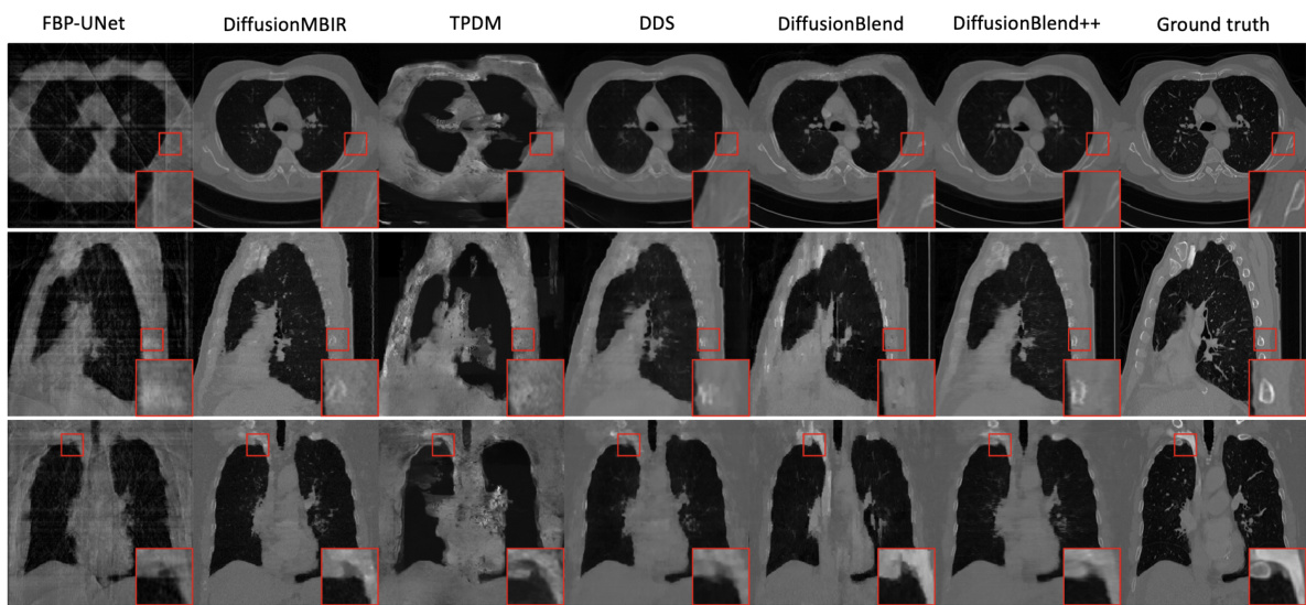
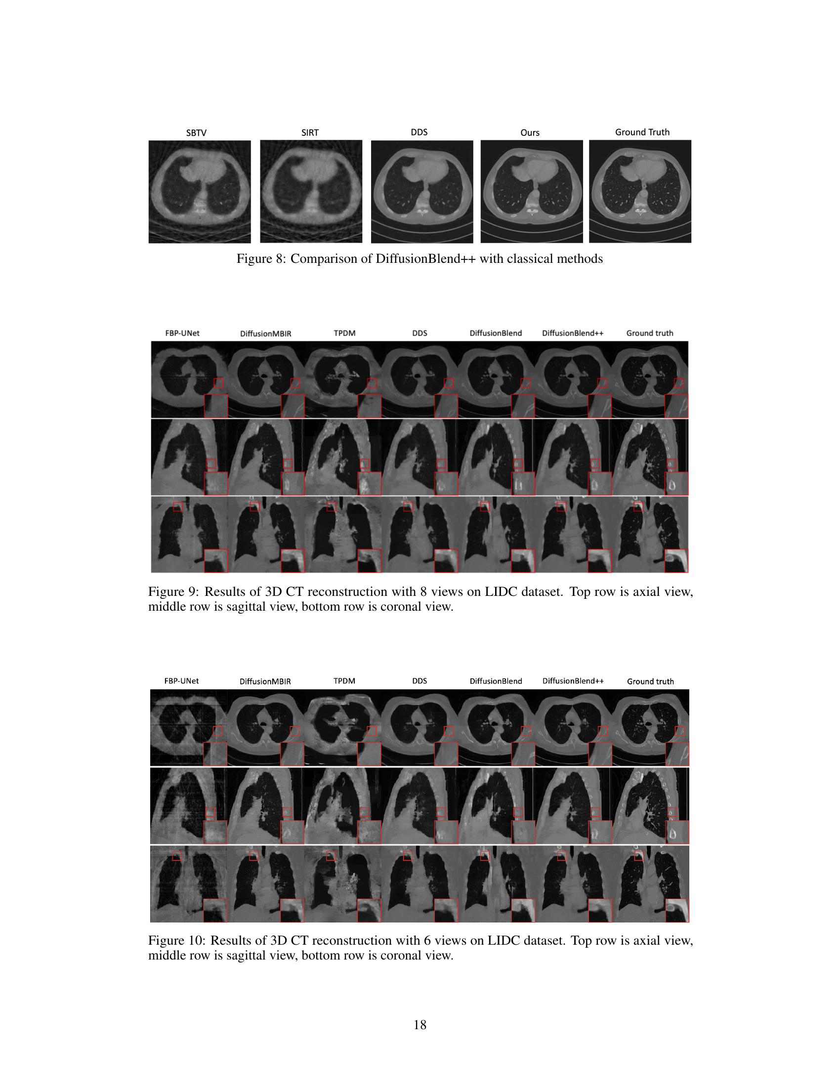
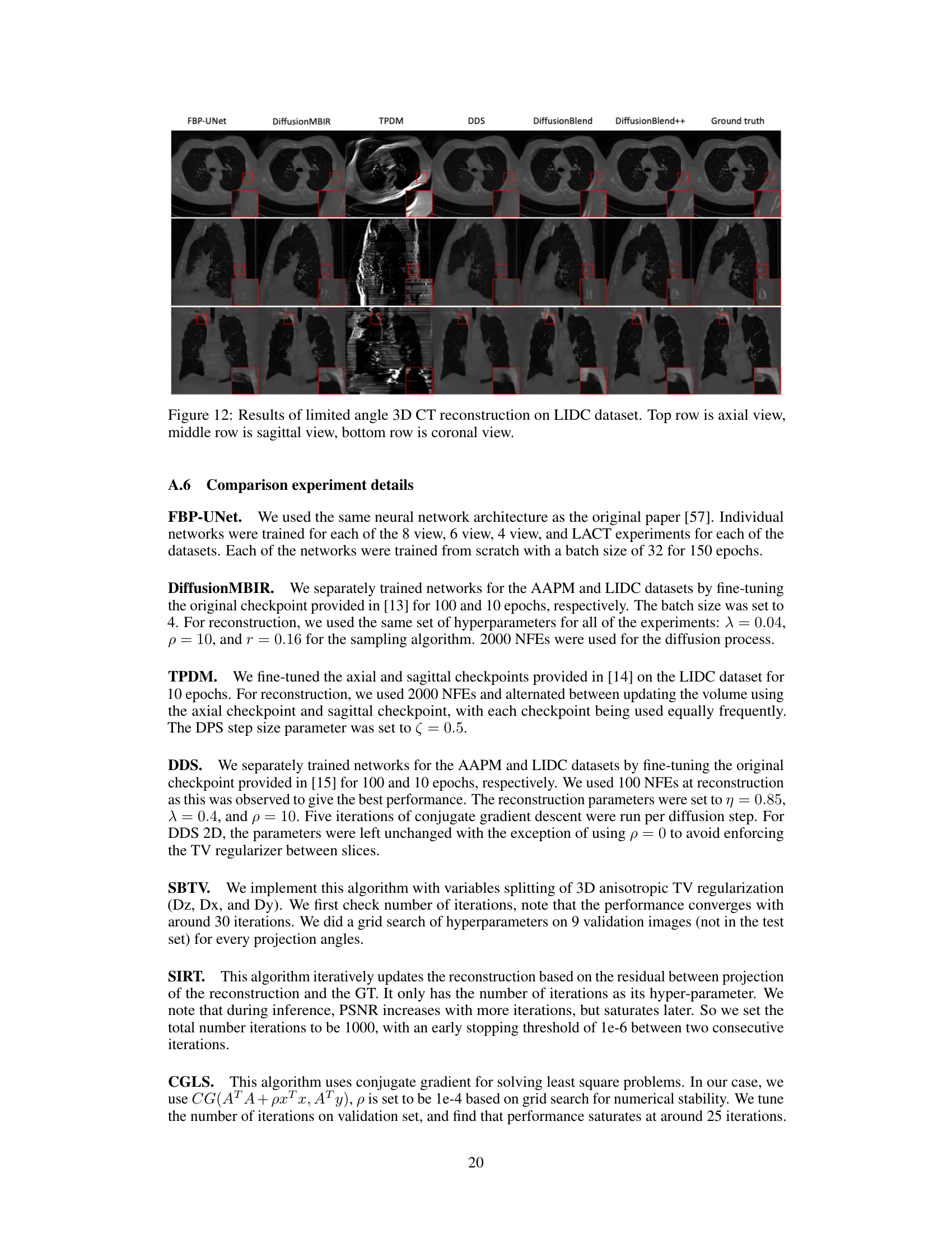
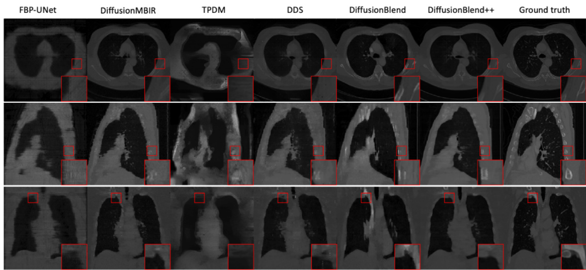
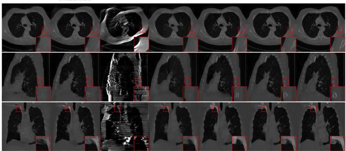
This figure shows a comparison of different CT reconstruction methods on the AAPM dataset using only 4 views. The top row displays axial slices of the reconstructed images. The methods compared include FBP (filtered back projection), FBP-UNet (a deep learning approach), DiffusionMBIR, DDS, DiffusionBlend and DiffusionBlend++. The ground truth is also included for reference. The image shows that DiffusionBlend++ produces results closest to the ground truth, demonstrating the effectiveness of the proposed method in reconstructing high-quality images even with limited data.
This figure displays the axial view of CT reconstruction results using different methods on the AAPM dataset with only 4 views. The methods compared include FBP, FBP-UNet, DDS, DDS 2D, and the proposed DiffusionBlend++. The ground truth is also included for reference. The figure shows the effectiveness of DiffusionBlend++ in reconstructing high-quality images even with a limited number of views, demonstrating improved image quality compared to the other methods.
This figure compares the results of CT reconstruction using different methods on the AAPM dataset with 4 views. The axial view of the CT scans is shown. The methods compared include FBP, FBP-UNet, DDS (2D), DDS, and the proposed DiffusionBlend++ method. The ground truth image is also shown for reference. The figure visually demonstrates the improved performance of DiffusionBlend++ compared to the other methods.
More on tables

This table presents a quantitative comparison of different methods for sparse-view computed tomography (CT) reconstruction. The metrics used are PSNR (Peak Signal-to-Noise Ratio) and SSIM (Structural Similarity Index). Results are shown for both the AAPM and LIDC datasets, and for different numbers of views (8, 6, and 4). The table highlights the superior performance of the proposed DiffusionBlend++ method.

This table presents a quantitative comparison of different methods for sparse-view computed tomography (CT) reconstruction on axial slices. It compares the performance of several methods, including FBP, FBP-UNet, DiffusionMBIR, TPDM, DDS 2D, DDS, DiffusionBlend, and DiffusionBlend++, across various metrics (PSNR and SSIM) and different numbers of views (4, 6, and 8) on two datasets (AAPM and LIDC). The best-performing methods for each metric and view count are highlighted in bold.

This table compares the performance of different methods for sparse-view CT reconstruction on the axial view using two datasets, AAPM and LIDC. The metrics used are PSNR and SSIM, both higher values indicating better reconstruction quality. The methods compared include traditional methods like FBP and FBP-UNet and several diffusion-based methods such as DiffusionMBIR, TPDM, and DDS. The table shows how DiffusionBlend++ achieves the best performance across different numbers of views and across the two datasets.

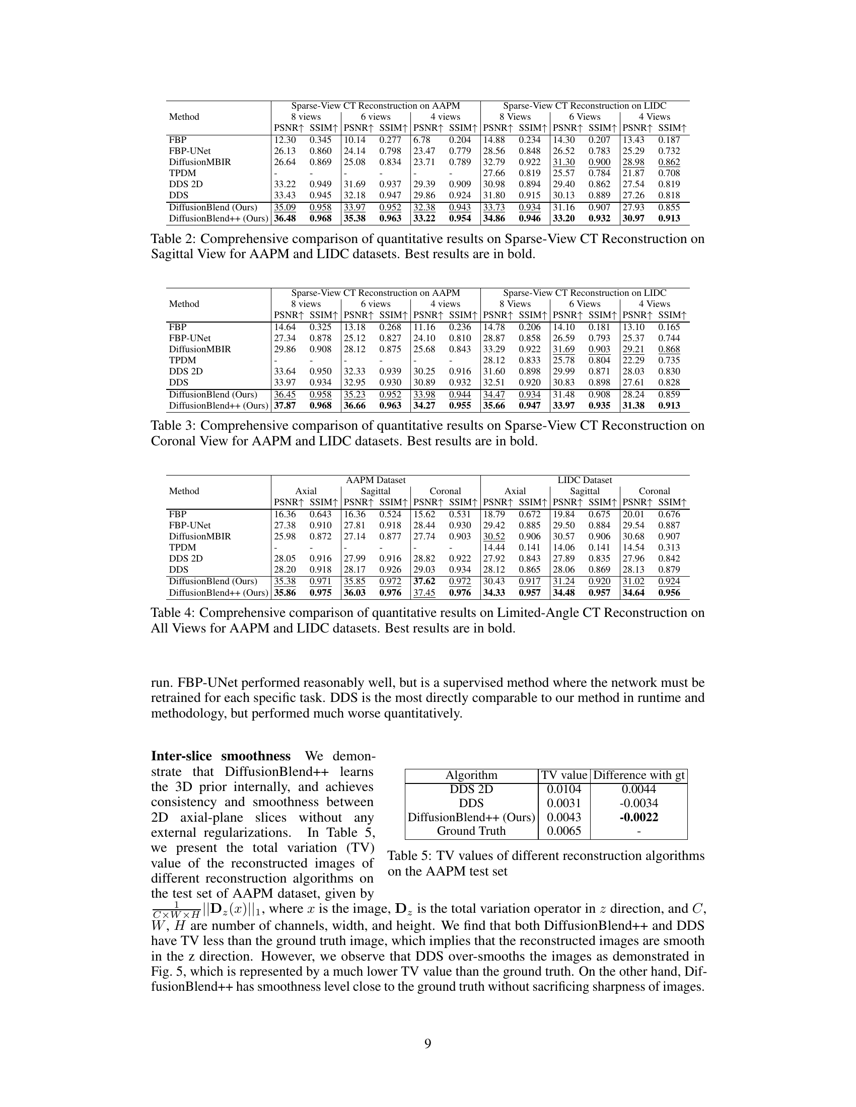
This table compares the total variation (TV) values of reconstructed images from different algorithms on the AAPM test dataset. The TV values represent the smoothness of the images, with lower values indicating smoother images. The table shows that DiffusionBlend++, the proposed method, achieves a TV value very close to the ground truth, indicating a good balance between smoothness and detail preservation. In contrast, DDS, another state-of-the-art method, over-smooths the images, resulting in a lower TV value than the ground truth.

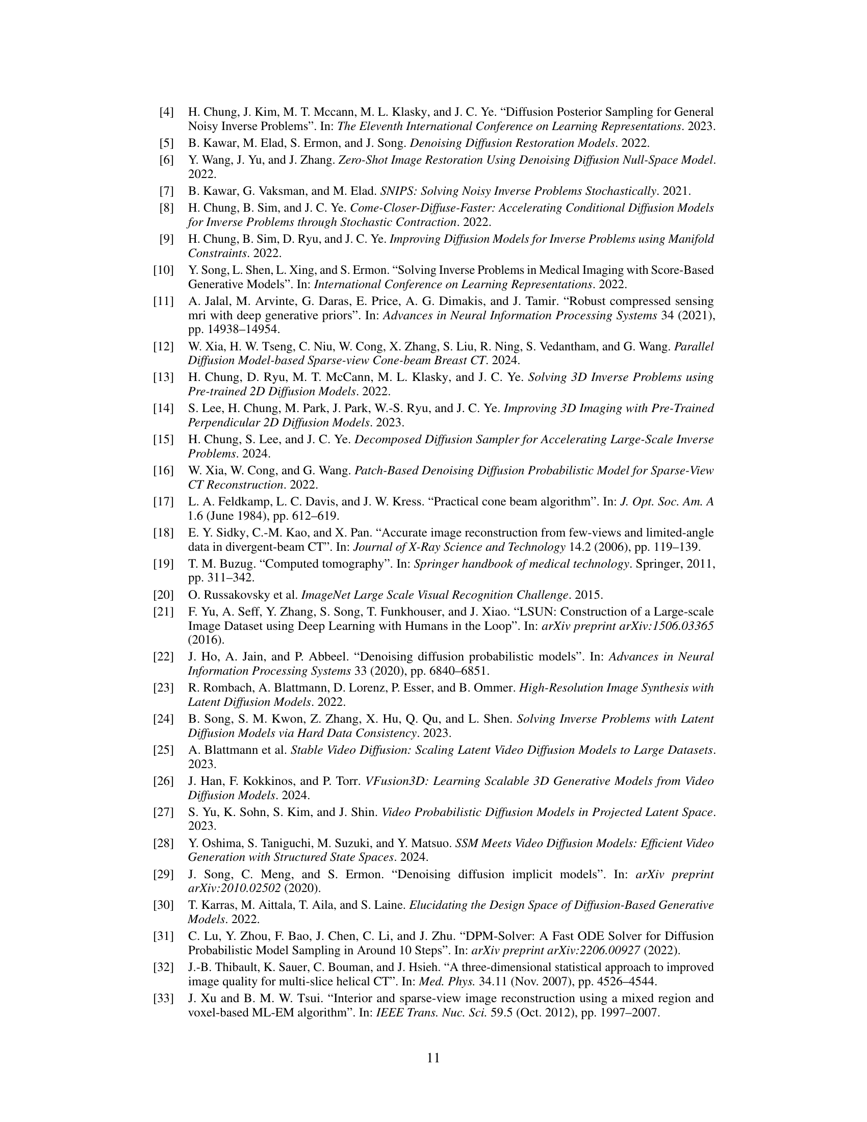
This table presents the results of an ablation study evaluating the impact of two blending modules on the performance of the DiffusionBlend++ method for 3D CT reconstruction. The study was conducted using the AAPM dataset, specifically focusing on sagittal view reconstructions. The table shows the PSNR and SSIM values achieved with different combinations of the adjacency-slice blending module and cross-slice blending module, demonstrating the contribution of each module to the overall performance improvement.

This table shows the effectiveness of adding adjacency-slice blending and cross-slice blending modules to the reverse sampling process in the DiffusionBlend++ model. It demonstrates that both the adjacency-slice blending and the cross-slice blending modules contribute to better reconstruction quality, as indicated by improvements in PSNR and SSIM.

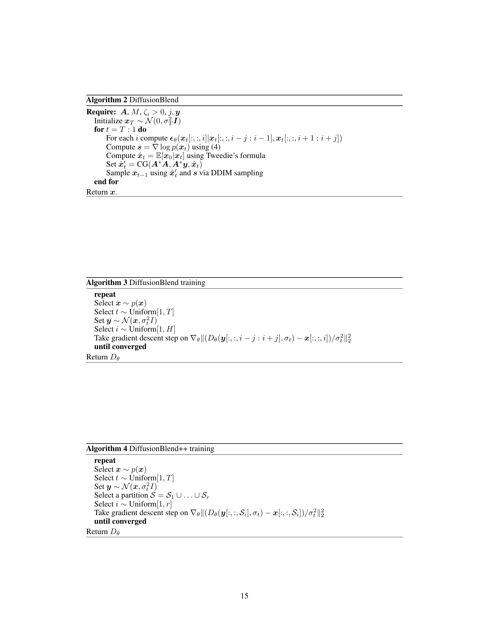
This table presents the Peak Signal-to-Noise Ratio (PSNR) values achieved by the DDS and DiffusionBlend++ methods for different numbers of neural function evaluations (NFEs) in the context of 8-view sparse-view computed tomography (SVCT) reconstruction. It highlights the impact of NFEs on reconstruction quality for both methods, showing DiffusionBlend++’s superior performance and robustness compared to DDS across various NFEs.

This table shows the Peak Signal-to-Noise Ratio (PSNR) results for 8-view sparse-view computed tomography (CT) reconstruction using DiffusionBlend++, varying the frequency of applying slice jumps during reconstruction. The frequency indicates how often the algorithm uses partitions with ‘jumping’ slices instead of adjacent slices. A frequency of 2 means that adjacent and jumping slices are used alternately, while a higher frequency means jumping slices are used less frequently.
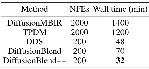
This table compares the wall clock time (in minutes) taken by different methods to reconstruct a 3D CT scan using 8 views. The methods compared include DiffusionMBIR, TPDM, DDS, DiffusionBlend, and DiffusionBlend++. The number of neural function evaluations (NFEs) used for each method is also listed. It demonstrates that DiffusionBlend++ achieves comparable or better reconstruction speed compared to other state-of-the-art methods.

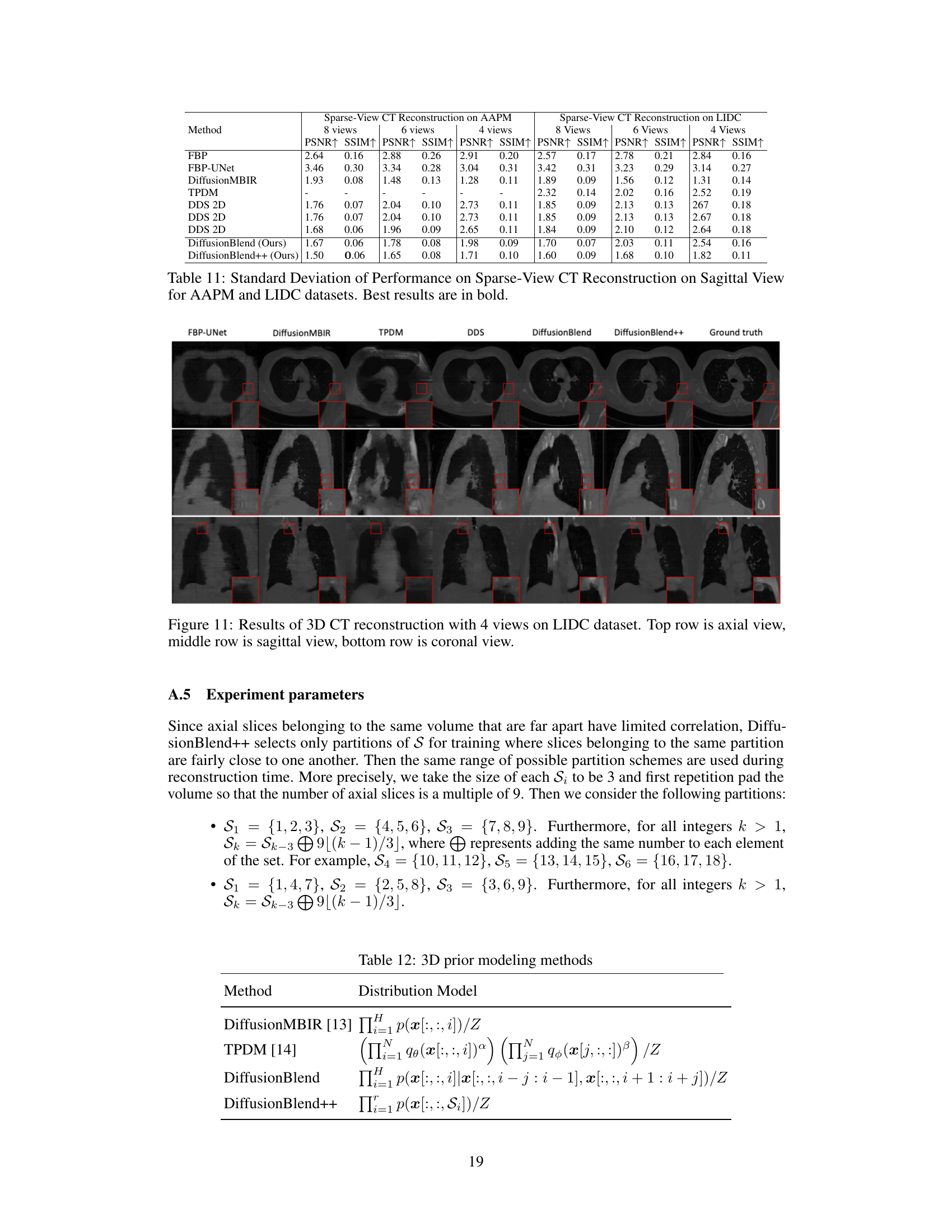
This table compares the performance of different methods for sparse-view CT reconstruction on axial slices of the AAPM and LIDC datasets. The methods compared include FBP, FBP-UNet, DiffusionMBIR, TPDM, DDS 2D, DDS, DiffusionBlend, and DiffusionBlend++. The table shows the PSNR and SSIM values for each method under different numbers of views (4, 6, and 8). Higher PSNR and SSIM values indicate better reconstruction quality. The best results for each metric and view are highlighted in bold.

This table compares the performance of different methods for sparse-view computed tomography (CT) reconstruction on two datasets: AAPM and LIDC. The performance is measured using Peak Signal-to-Noise Ratio (PSNR) and Structural Similarity Index (SSIM). The table shows the results for different numbers of views (4, 6, and 8) used in the reconstruction process. Higher PSNR and SSIM values indicate better reconstruction quality.
Full paper#

