TL;DR#
Training high-fidelity 3D models for large-scale scenes is computationally expensive, posing a major challenge for real-time applications like autonomous driving and virtual reality. Existing methods like 3D Gaussian Splatting struggle with the memory and computational requirements of handling massive datasets. Furthermore, simply dividing the scene into smaller blocks and training separate models for each is not efficient, as it necessitates querying multiple sub-models during inference which is slow.
The proposed method, DOGS, tackles this problem by distributing the training process across multiple machines using an alternating direction method of multipliers (ADMM). This allows for parallel processing and significant speedup (6+ times faster). Crucially, DOGS maintains a global model on a master node, with local models on slave nodes that converge to the global model, guaranteeing consistency. This leads to significant time savings without compromising the final rendering quality. The method showcases state-of-the-art rendering quality on various large-scale datasets, demonstrating its practical effectiveness for real-world applications.
Key Takeaways#
Why does it matter?#
This paper is crucial for researchers working on large-scale 3D reconstruction and neural rendering. It significantly advances the training efficiency of 3D Gaussian Splatting, a leading method for high-fidelity 3D scene representation, enabling faster and more scalable scene reconstruction for large-scale applications. This opens new avenues for research in distributed training algorithms and their application to other computationally intensive tasks in computer vision and graphics.
Visual Insights#

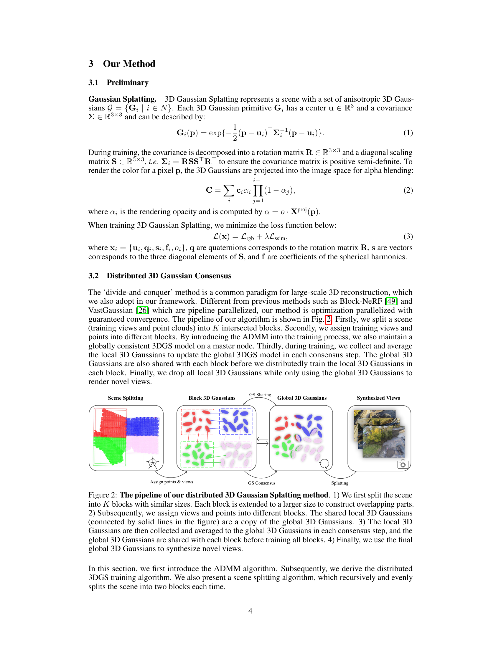
🔼 This figure illustrates the pipeline of the proposed DOGS method for distributed 3D Gaussian splatting. It shows how a scene is divided into blocks, how local and global 3D Gaussian models are maintained and updated through consensus, and how the final global model is used for rendering.
read the caption
Figure 2: The pipeline of our distributed 3D Gaussian Splatting method. 1) We first split the scene into K blocks with similar sizes. Each block is extended to a larger size to construct overlapping parts. 2) Subsequently, we assign views and points into different blocks. The shared local 3D Gaussians (connected by solid lines in the figure) are a copy of the global 3D Gaussians. 3) The local 3D Gaussians are then collected and averaged to the global 3D Gaussians in each consensus step, and the global 3D Gaussians are shared with each block before training all blocks. 4) Finally, we use the final global 3D Gaussians to synthesize novel views.

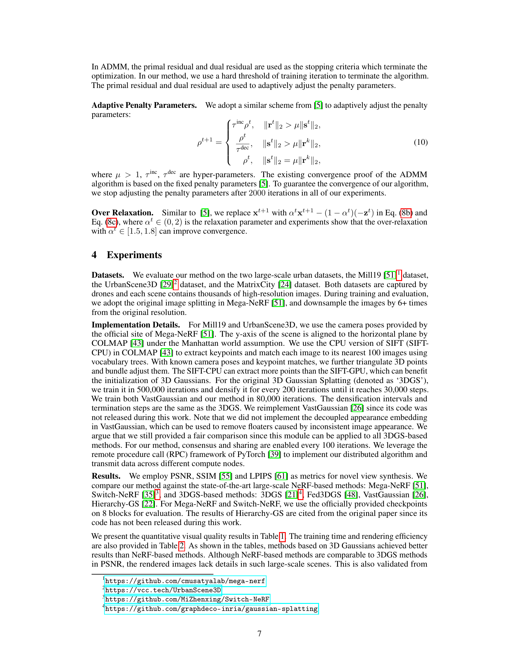
🔼 This table presents a quantitative comparison of different methods for novel view synthesis on two large-scale urban datasets: Mill19 and UrbanScene3D. The metrics used are PSNR (Peak Signal-to-Noise Ratio), SSIM (Structural Similarity Index), and LPIPS (Learned Perceptual Image Patch Similarity). Higher PSNR and SSIM values indicate better image quality, while a lower LPIPS value signifies better perceptual similarity. The table highlights the best performing method (red), second best (orange), and third best (yellow) for each scene. A dagger symbol (†) denotes results obtained without applying decoupled appearance encoding, allowing for a fair comparison between methods with and without this technique.
read the caption
Table 1: Quantitative results of novel view synthesis on Mill19 [51] dataset and Urban-Scene3D [29] dataset. ↑: higher is better, ↓: lower is better. The red, orange and yellow colors respectively denote the best, the second best, and the third best results. † denotes without applying the decoupled appearance encoding.
In-depth insights#
Distributed 3DGS#
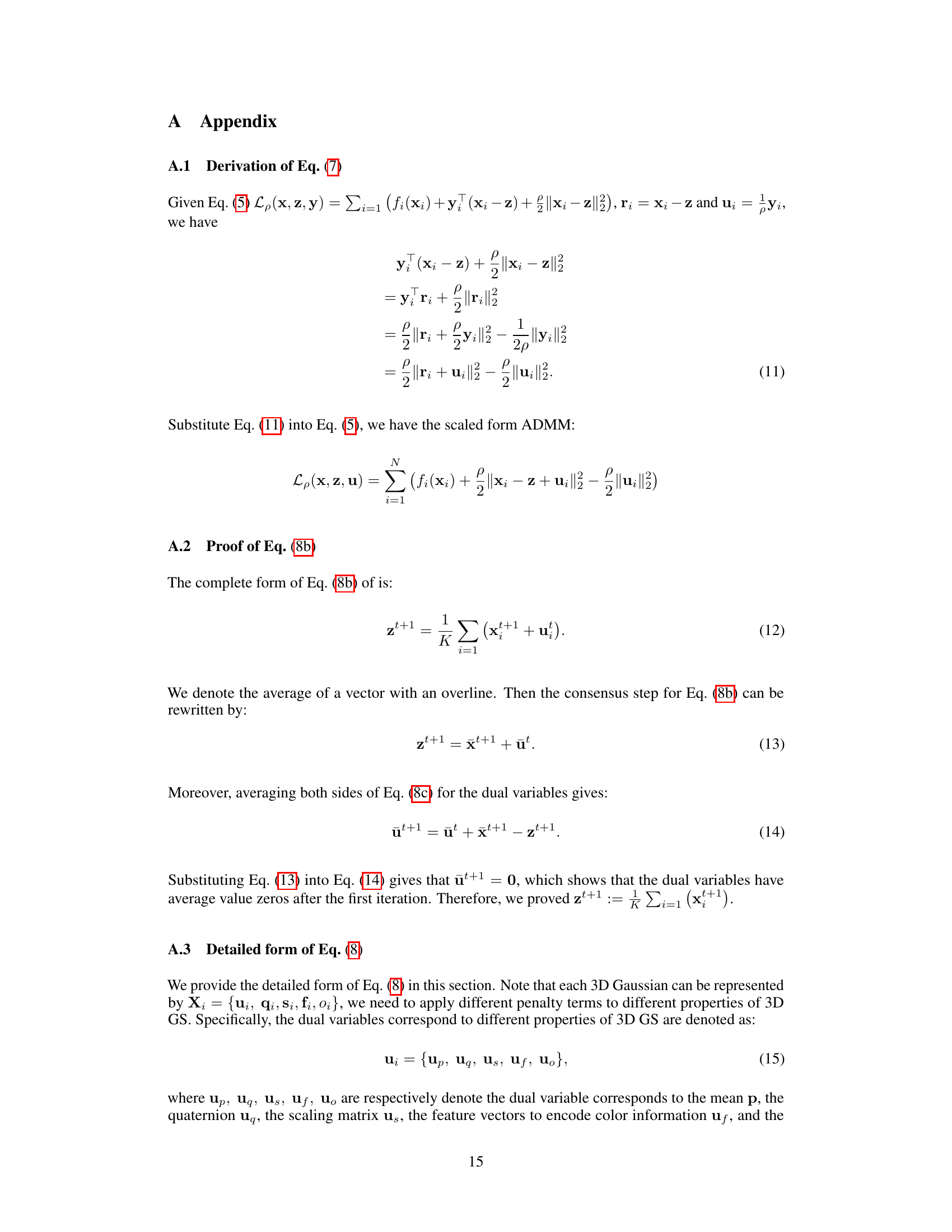
The concept of “Distributed 3DGS” presents a compelling approach to address the limitations of traditional 3D Gaussian Splatting (3DGS) methods when dealing with large-scale 3D reconstruction. By distributing the training process, the method aims to overcome GPU memory constraints that often hinder the processing of massive datasets. This distribution is achieved by dividing the scene into smaller blocks and processing each block on separate computational units. A key aspect is ensuring consistency across these independently trained blocks; techniques like Alternating Direction Method of Multipliers (ADMM) are likely employed to maintain a coherent global model from the individual block models, improving convergence and stability. Maintaining a global model during inference offers the advantage of simpler query processes, avoiding the computational complexity of querying multiple models inherent in other large-scale approaches. However, this distributed training strategy introduces challenges, notably the need for efficient communication and synchronization among computing units to maintain data consistency. The success of the method hinges on carefully balancing the computational workload and the overhead of inter-unit communication.
ADMM for 3DGS#
Applying the Alternating Direction Method of Multipliers (ADMM) to 3D Gaussian Splatting (3DGS) for large-scale 3D reconstruction presents a compelling approach to distributed training. ADMM’s ability to decompose a large problem into smaller, manageable subproblems aligns well with the inherent challenges of processing massive 3D Gaussian datasets. By distributing the scene into blocks and using ADMM, we can parallelize the computation, significantly reducing training time while preserving overall model consistency. The global model acts as a central reference point, ensuring that the local models trained on individual blocks converge towards a unified representation of the scene. This method cleverly balances computational efficiency with the need to maintain a high-fidelity global model for superior rendering quality. However, challenges remain, such as effectively handling communication overhead between the master node and slave nodes during the consensus step. The method’s reliance on a master node could also become a bottleneck as the scale of the problem increases. Despite these challenges, the application of ADMM to 3DGS demonstrates a promising avenue for overcoming the computational constraints typically associated with large-scale 3D reconstruction.
Recursive Scene Split#
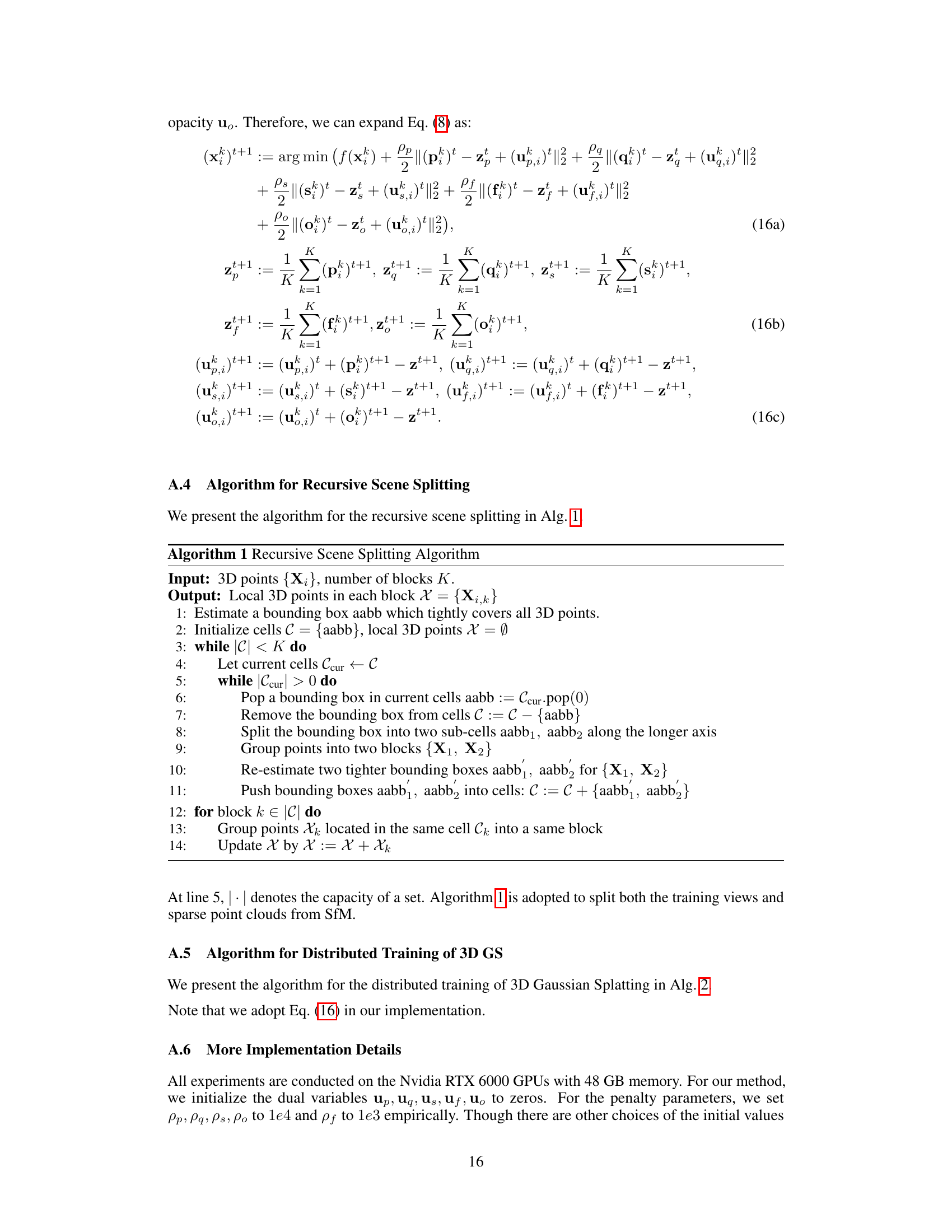
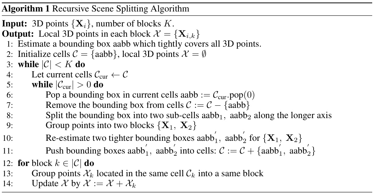
The concept of “Recursive Scene Split” in large-scale 3D reconstruction is crucial for managing computational complexity. It’s a divide-and-conquer strategy that recursively subdivides a large scene into smaller, more manageable blocks. This approach directly addresses the memory limitations of processing massive datasets. Recursive splitting ensures that each block is roughly equal in size, preventing some blocks from becoming overly large and computationally expensive. It also facilitates balanced parallel processing which is essential for efficiency. The method’s effectiveness hinges on the choice of splitting criteria and the way overlapping regions between adjacent blocks are handled; it balances the need for efficient processing with the necessity to maintain scene consistency. The tradeoff is between computational load per block and communication/synchronization overhead to maintain the global scene structure. A well-designed recursive split ensures faster processing, improved convergence and better memory management. Careful consideration must be given to ensuring that the overlapping regions are large enough for training convergence, yet small enough to limit unnecessary redundancy and communication.
Convergence Rate#
The convergence rate in distributed training of large-scale 3D Gaussian splatting is a critical factor determining the overall efficiency. The authors cleverly leverage the Alternating Direction Method of Multipliers (ADMM) to ensure consistency across distributed blocks. However, ADMM’s sensitivity to parameter initialization necessitates strategies to improve convergence. The adaptive penalty parameter scheme dynamically adjusts parameters based on primal and dual residuals, enhancing stability and speed. Over-relaxation further accelerates convergence, allowing the method to reach a solution faster. Despite these improvements, scene splitting strategies and the number of blocks significantly impact training time. Achieving a balance between block size uniformity and sufficient overlap to facilitate information sharing between blocks remains a challenge. Further research exploring optimal splitting methods and adaptive penalty parameter schedules could further boost convergence, enhancing the scalability and practical applicability of distributed 3DGS.
Future Work#
The paper’s ‘Future Work’ section suggests several promising avenues. Addressing the GPU memory limitations imposed by large-scale scenes is crucial, potentially through level-of-detail (LOD) techniques to reduce the number of 3D Gaussians processed. Improving the flexibility of the distributed training approach is another key area. While the proposed method delivers speedups, its reliance on a central master node limits scalability and flexibility. Exploring fully decentralized alternatives would enhance usability and applicability. Finally, extending the method to handle various 3D Gaussian representations and integrating advanced features like dynamic scenes or appearance changes would significantly broaden its impact. Incorporating techniques for handling various data formats and noise levels to enhance robustness and further optimize performance are also valuable avenues for exploration.
More visual insights#
More on figures

🔼 This figure illustrates the pipeline of the proposed DOGS method. The scene is first split into K blocks with overlapping regions. Each block has its own set of local 3D Gaussians. During training, these local 3D Gaussians are iteratively updated, and their averages are used to update a global 3D Gaussian model. The global model is then shared with all blocks to maintain consistency. After training, only the global model is used for rendering novel views.
read the caption
Figure 2: The pipeline of our distributed 3D Gaussian Splatting method. 1) We first split the scene into K blocks with similar sizes. Each block is extended to a larger size to construct overlapping parts. 2) Subsequently, we assign views and points into different blocks. The shared local 3D Gaussians (connected by solid lines in the figure) are a copy of the global 3D Gaussians. 3) The local 3D Gaussians are then collected and averaged to the global 3D Gaussians in each consensus step, and the global 3D Gaussians are shared with each block before training all blocks. 4) Finally, we use the final global 3D Gaussians to synthesize novel views.

🔼 This figure illustrates the steps involved in the distributed 3D Gaussian Splatting process. The scene is first divided into K blocks with overlapping regions to ensure data consistency between neighboring blocks. Views and points are assigned to their respective blocks. Then, a global 3D Gaussian model is maintained on a master node. Local models are updated iteratively. Local 3D Gaussians are shared and averaged to update the global model, which is then re-distributed. Finally, only the global model is used for rendering.
read the caption
Figure 2: The pipeline of our distributed 3D Gaussian Splatting method. 1) We first split the scene into K blocks with similar sizes. Each block is extended to a larger size to construct overlapping parts. 2) Subsequently, we assign views and points into different blocks. The shared local 3D Gaussians (connected by solid lines in the figure) are a copy of the global 3D Gaussians. 3) The local 3D Gaussians are then collected and averaged to the global 3D Gaussians in each consensus step, and the global 3D Gaussians are shared with each block before training all blocks. 4) Finally, we use the final global 3D Gaussians to synthesize novel views.
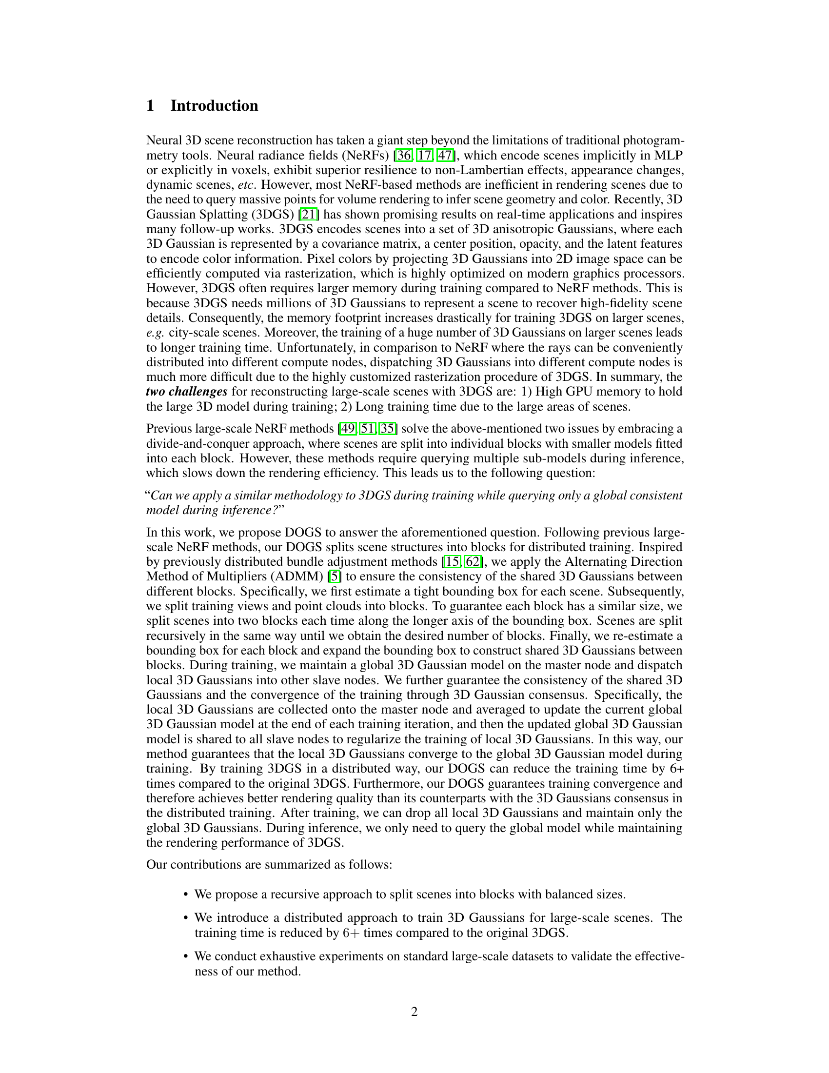
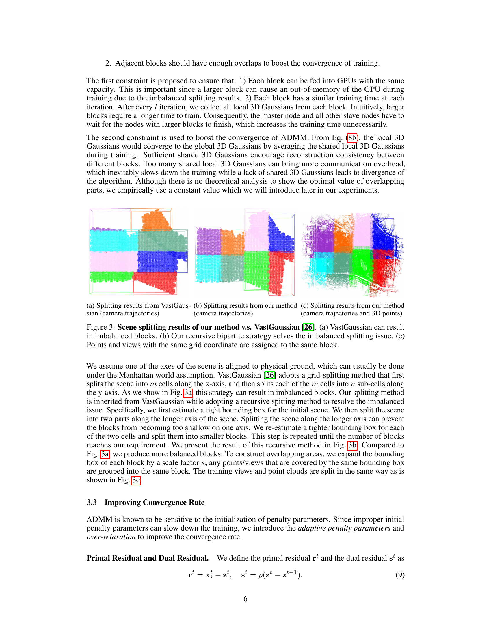
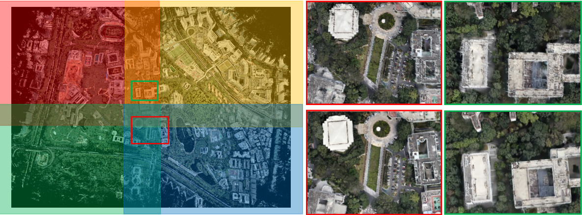
🔼 This figure shows a comparison of the results obtained using the proposed DOGS method and the original 3D Gaussian Splatting (3D GS) method for 3D reconstruction on the large-scale UrbanScene3D dataset. The top row displays the 3D Gaussian primitives used to represent the scene, showing 8.27 million primitives in the DOGS method. The bottom row shows rendered images generated from those primitives, highlighting the improved rendering quality achieved using the DOGS method. The figure demonstrates that the DOGS method significantly accelerates the training process of 3D GS while maintaining high rendering quality.
read the caption
Figure 1: DOGS accelerates 3D GS training on large-scale UrbanScene3D dataset [29] by 6+ times with better rendering quality. Top: 3D Gaussian primitives (8.27M); Bottom: rendered images.
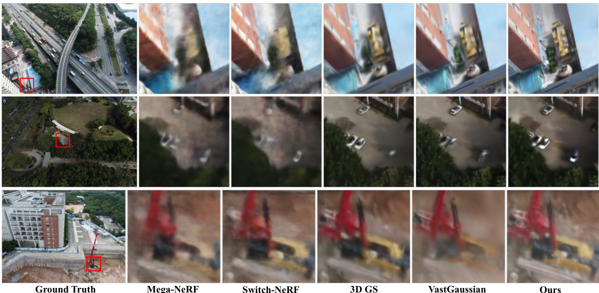
🔼 This figure shows the results of applying the DOGS method to the UrbanScene3D dataset. The top row displays 8.27 million 3D Gaussian primitives that represent the 3D scene reconstructed by DOGS. The bottom row shows the rendered images generated from these primitives, demonstrating the high-fidelity rendering quality achieved by the method. The caption highlights that DOGS accelerates the training process by more than 6 times compared to standard 3D Gaussian Splatting.
read the caption
Figure 1: DOGS accelerates 3D GS training on large-scale UrbanScene3D dataset [29] by 6+ times with better rendering quality. Top: 3D Gaussian primitives (8.27M); Bottom: rendered images.

🔼 This figure shows the results of applying DOGS to the UrbanScene3D dataset. The top row displays 8.27 million 3D Gaussian primitives used to represent the scene. The bottom row shows rendered images generated from these primitives, highlighting the improved rendering quality achieved by DOGS. The caption also emphasizes that DOGS speeds up training by more than 6 times compared to the original 3D Gaussian Splatting method.
read the caption
Figure 1: DOGS accelerates 3D GS training on large-scale UrbanScene3D dataset [29] by 6+ times with better rendering quality. Top: 3D Gaussian primitives (8.27M); Bottom: rendered images.
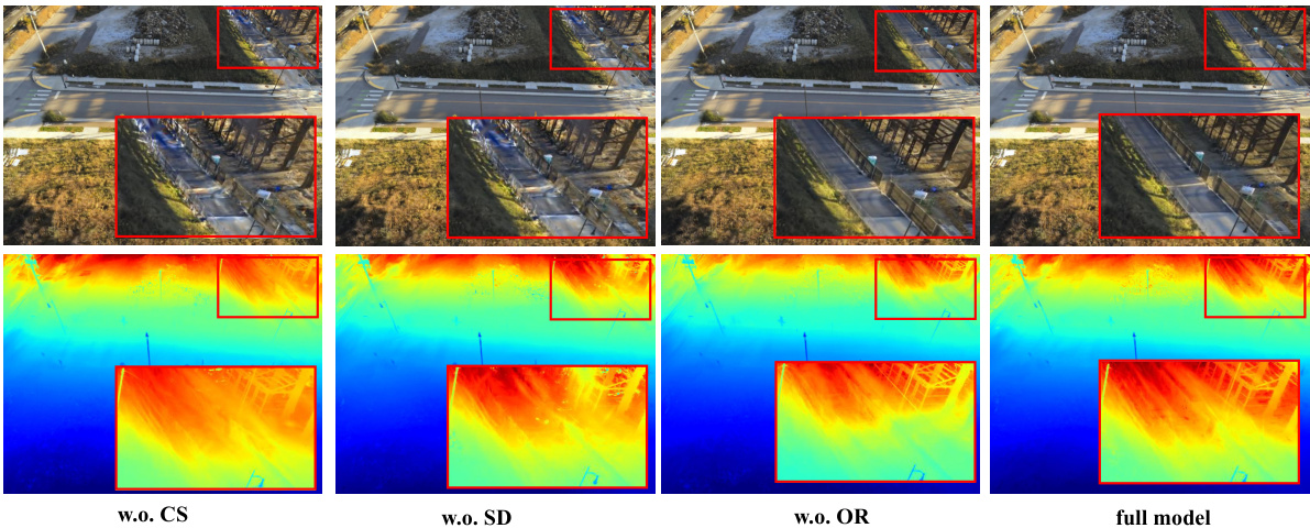
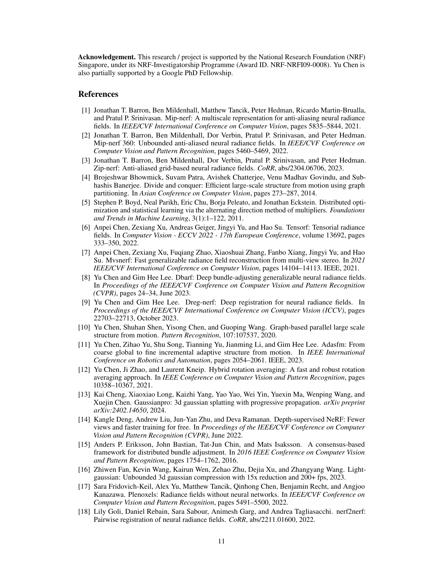
🔼 This figure shows the results of an ablation study comparing different versions of the DOGS method. The top row displays rendered images, while the bottom row shows the corresponding depth maps. The variations compared include versions without consensus (w.o. CS), without self-adaptation (w.o. SD), without over-relaxation (w.o. OR), and the full model. Red boxes highlight areas where differences are most apparent.
read the caption
Figure 7: Ablation study of our method. Top: rendered images; Bottom: rendered depths.

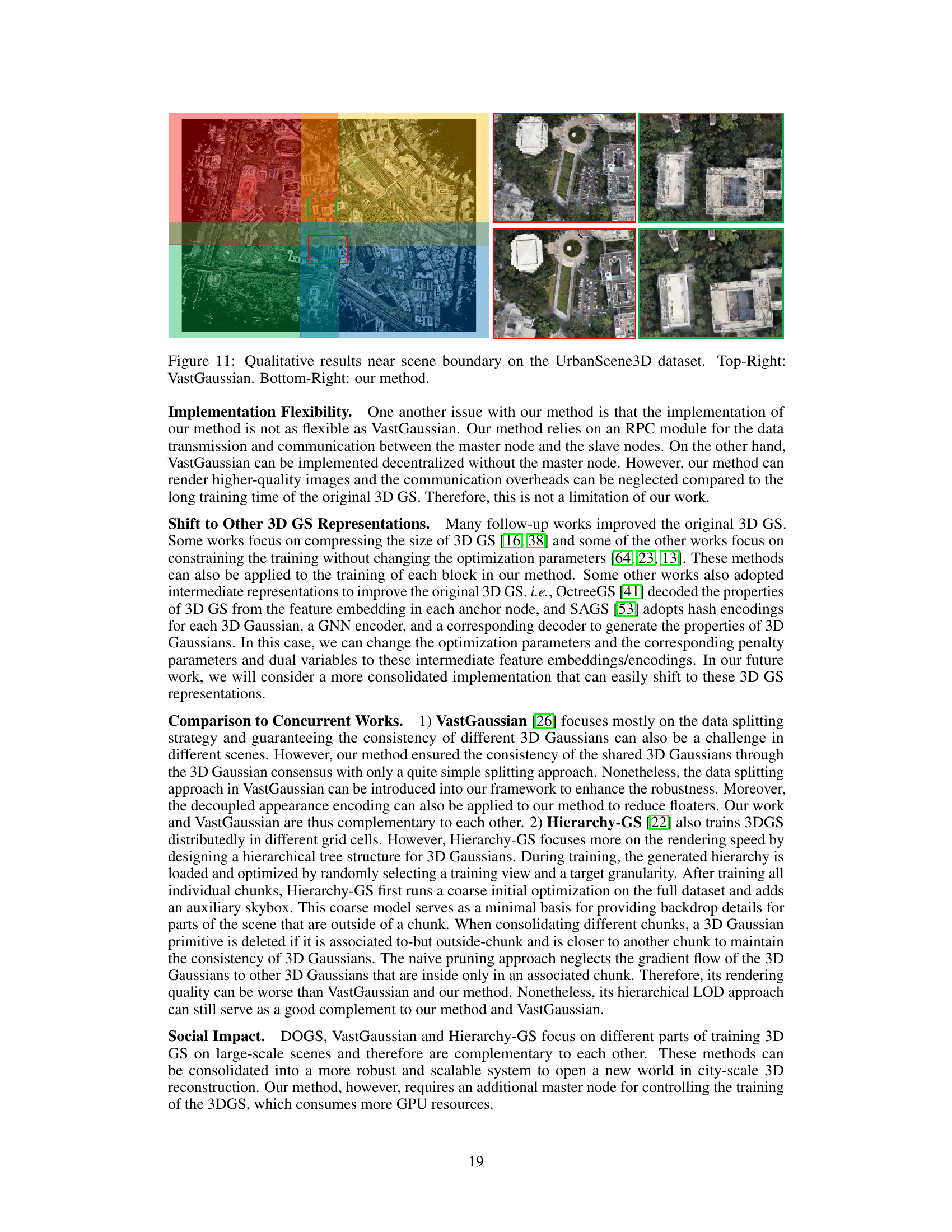
🔼 This figure shows a comparison of the results with and without the consensus step. The red boxes highlight the areas near the boundary between blocks. The results without consensus steps show obvious artifacts near the boundary, which indicates that the consensus step is important for ensuring the consistency of the global 3D Gaussian model.
read the caption
Figure 8: Importance of the consensus step.
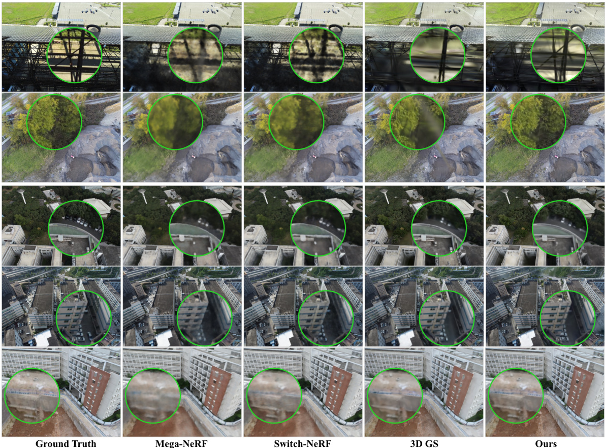
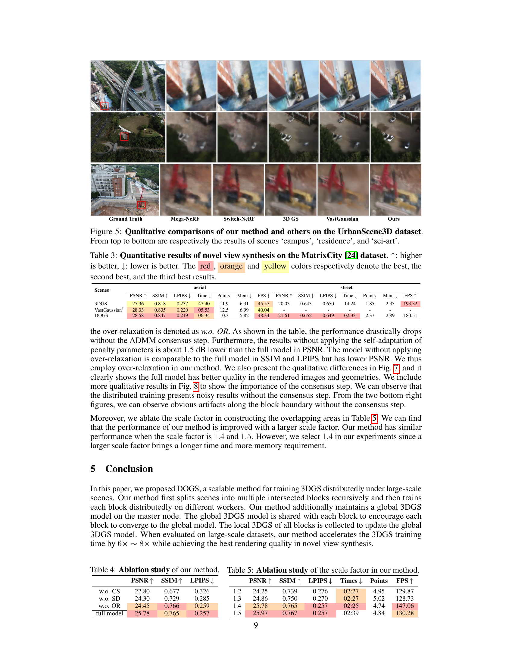
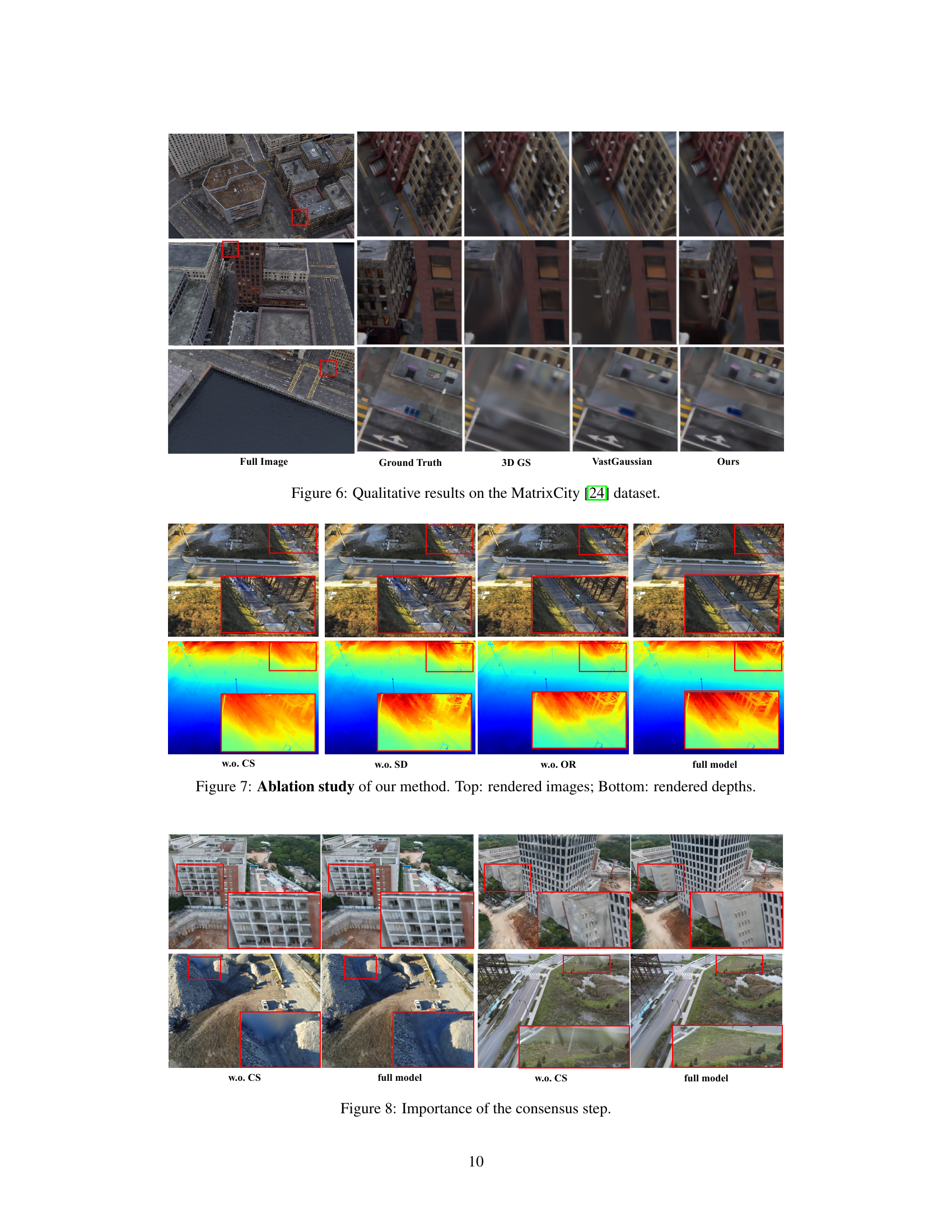
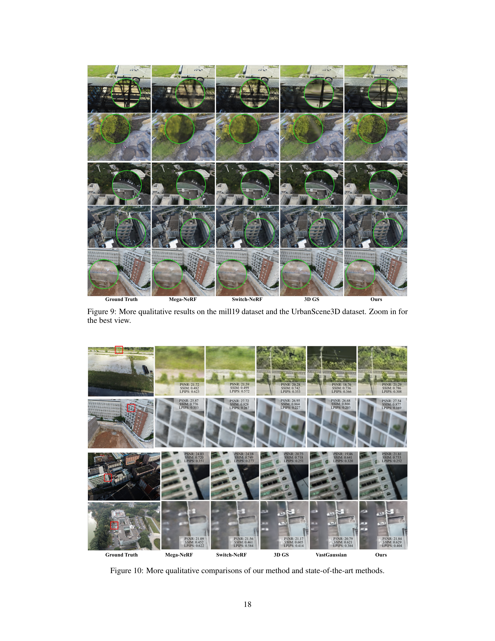
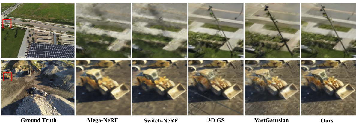
🔼 This figure presents a qualitative comparison of the proposed DOGS method against several state-of-the-art methods, including Mega-NeRF, Switch-NeRF, and the original 3D GS, on various scenes. Green circles highlight areas for closer examination. The comparison focuses on the visual quality of novel view synthesis, showing the superior detail and clarity achieved by the proposed method. It demonstrates the impact of distributed training and consensus on large-scale scenes.
read the caption
Figure 10: More qualitative comparisons of our method and state-of-the-art methods.
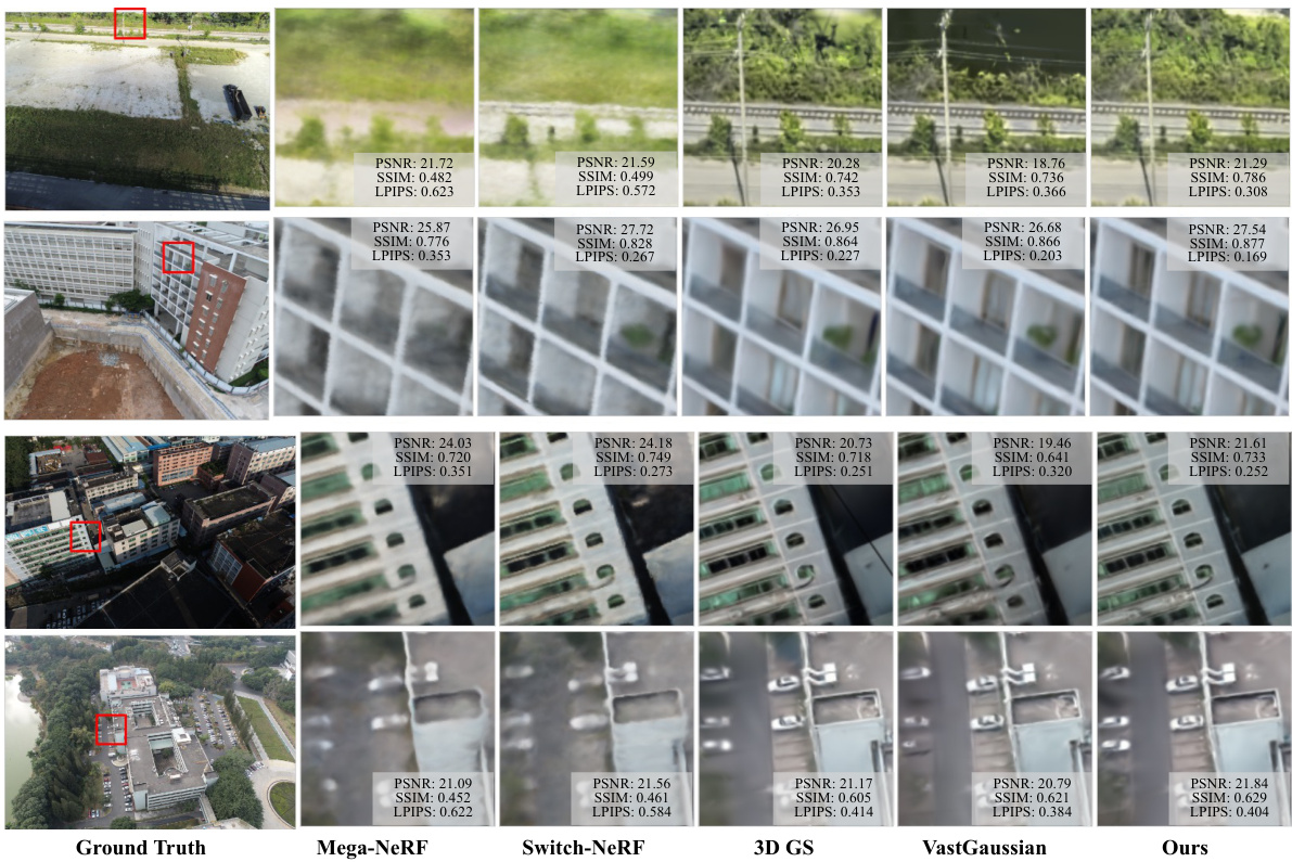
🔼 This figure illustrates the pipeline of the DOGS method. It shows how the scene is divided into blocks, local and global 3D Gaussian models are trained and updated in an alternating fashion using ADMM, and finally, how only the global model is used for inference. The figure highlights the key steps: scene splitting, Gaussian sharing, consensus, and synthesis.
read the caption
Figure 2: The pipeline of our distributed 3D Gaussian Splatting method. 1) We first split the scene into K blocks with similar sizes. Each block is extended to a larger size to construct overlapping parts. 2) Subsequently, we assign views and points into different blocks. The shared local 3D Gaussians (connected by solid lines in the figure) are a copy of the global 3D Gaussians. 3) The local 3D Gaussians are then collected and averaged to the global 3D Gaussians in each consensus step, and the global 3D Gaussians are shared with each block before training all blocks. 4) Finally, we use the final global 3D Gaussians to synthesize novel views.
🔼 This figure illustrates the pipeline of the DOGS method for distributed 3D Gaussian splatting. It shows how the scene is divided into blocks, how local and global 3D Gaussian models are maintained and updated through consensus, and how the final global model is used for rendering.
read the caption
Figure 2: The pipeline of our distributed 3D Gaussian Splatting method. 1) We first split the scene into K blocks with similar sizes. Each block is extended to a larger size to construct overlapping parts. 2) Subsequently, we assign views and points into different blocks. The shared local 3D Gaussians (connected by solid lines in the figure) are a copy of the global 3D Gaussians. 3) The local 3D Gaussians are then collected and averaged to the global 3D Gaussians in each consensus step, and the global 3D Gaussians are shared with each block before training all blocks. 4) Finally, we use the final global 3D Gaussians to synthesize novel views.
More on tables

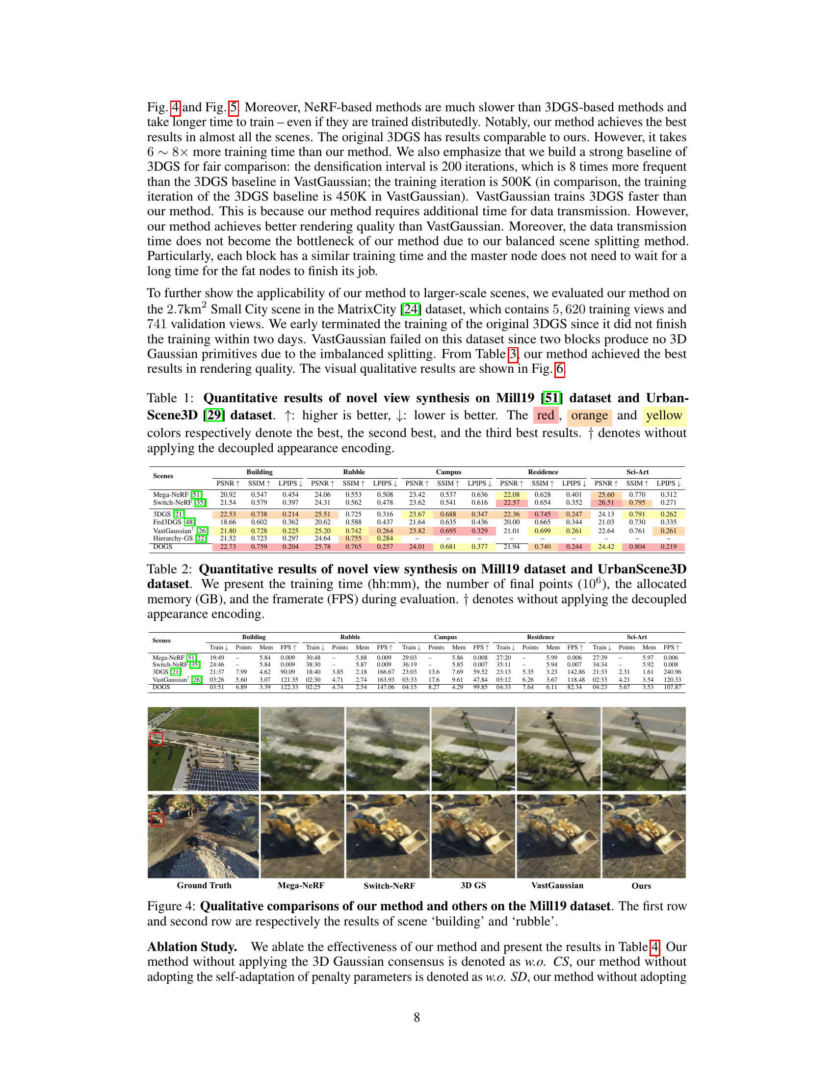
🔼 This table presents a quantitative comparison of different methods for novel view synthesis on the Mill19 and UrbanScene3D datasets. It shows the training time, the number of final 3D Gaussian points, the memory used during training and the frames per second (FPS) achieved during evaluation. The results help to assess the efficiency and quality of various methods in reconstructing and rendering large-scale scenes.
read the caption
Table 2: Quantitative results of novel view synthesis on Mill19 dataset and UrbanScene3D dataset. We present the training time (hh:mm), the number of final points (106), the allocated memory (GB), and the framerate (FPS) during evaluation. † denotes without applying the decoupled appearance encoding.

🔼 This table presents a quantitative comparison of the proposed DOGS method against several state-of-the-art methods for novel view synthesis on the MatrixCity dataset. It shows the PSNR, SSIM, and LPIPS metrics for both aerial and street views, along with training time, the number of points used in the final model, memory usage, and frames per second (FPS). Higher PSNR and SSIM values, and lower LPIPS values indicate better performance. The table also highlights the best-performing method for each metric in each scene type with color-coding.
read the caption
Table 3: Quantitative results of novel view synthesis on the MatrixCity [24] dataset. ↑: higher is better, ↓: lower is better. The red, orange and yellow colors respectively denote the best, the second best, and the third best results.

🔼 This table presents the ablation study of the proposed DOGS method. It shows the quantitative results (PSNR, SSIM, LPIPS) of novel view synthesis on the Mill19 and UrbanScene3D datasets when different components of the method are removed. The results are compared against the full model, showing the impact of the 3D Gaussian consensus (CS), self-adaptive penalty parameters (SD), and over-relaxation (OR) on the overall performance.
read the caption
Table 4: Ablation study of our method.
🔼 This table presents a quantitative comparison of different methods for novel view synthesis on two large-scale urban datasets: Mill19 and UrbanScene3D. The metrics used are PSNR, SSIM, and LPIPS. The table highlights the best performing method (DOGS) across various scenes within each dataset, indicating superior performance in terms of image quality. The notation for higher is better and lower is better is provided, along with color-coding to visually represent ranking of performance. The note indicates that some results exclude the decoupled appearance encoding technique.
read the caption
Table 1: Quantitative results of novel view synthesis on Mill19 [51] dataset and Urban-Scene3D [29] dataset. ↑: higher is better, ↓: lower is better. The red, orange and yellow colors respectively denote the best, the second best, and the third best results. † denotes without applying the decoupled appearance encoding.

🔼 This table presents a quantitative comparison of different methods for novel view synthesis on two large-scale datasets (Mill19 and UrbanScene3D). It shows the training time, the number of 3D Gaussian points used in the final model, the memory used (in GB), and the rendering speed (frames per second) achieved by each method. The results highlight the efficiency and quality of DOGS compared to other state-of-the-art techniques.
read the caption
Table 2: Quantitative results of novel view synthesis on Mill19 dataset and UrbanScene3D dataset. We present the training time (hh:mm), the number of final points (106), the allocated memory (GB), and the framerate (FPS) during evaluation. † denotes without applying the decoupled appearance encoding.
Full paper#
