Enhancing Robustness in Deep Reinforcement Learning: A Lyapunov Exponent Approach

↗ OpenReview ↗ NeurIPS Homepage ↗ Chat

TL;DR

#

Key Takeaways

#

Why does it matter?

#

This paper is crucial because it addresses the critical challenge of robustness in deep reinforcement learning (RL), a major obstacle to real-world applications. By introducing a novel Lyapunov Exponent regularisation, it offers a practical solution to improve the stability and reliability of RL agents, opening new avenues for research and development in this field. The findings are relevant to researchers working on control systems, robotics, and other areas where robust and reliable AI systems are required.

Visual Insights

#

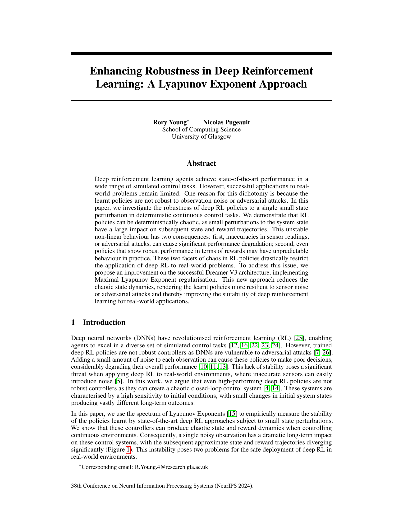
This figure shows the impact of a small perturbation in the initial state of a deterministic Walker Walk environment controlled by a trained Soft Actor-Critic agent. Three nearly identical simulations are run, differing only by a tiny change ( ±5 × 10-4 degrees) in the initial torso angle. Despite this minuscule difference, the reward and state trajectories diverge significantly after only 50 steps, illustrating the chaotic sensitivity of the system to initial conditions. This highlights a key challenge in applying deep reinforcement learning to real-world scenarios, where sensor noise or other small disturbances can lead to drastically different outcomes.

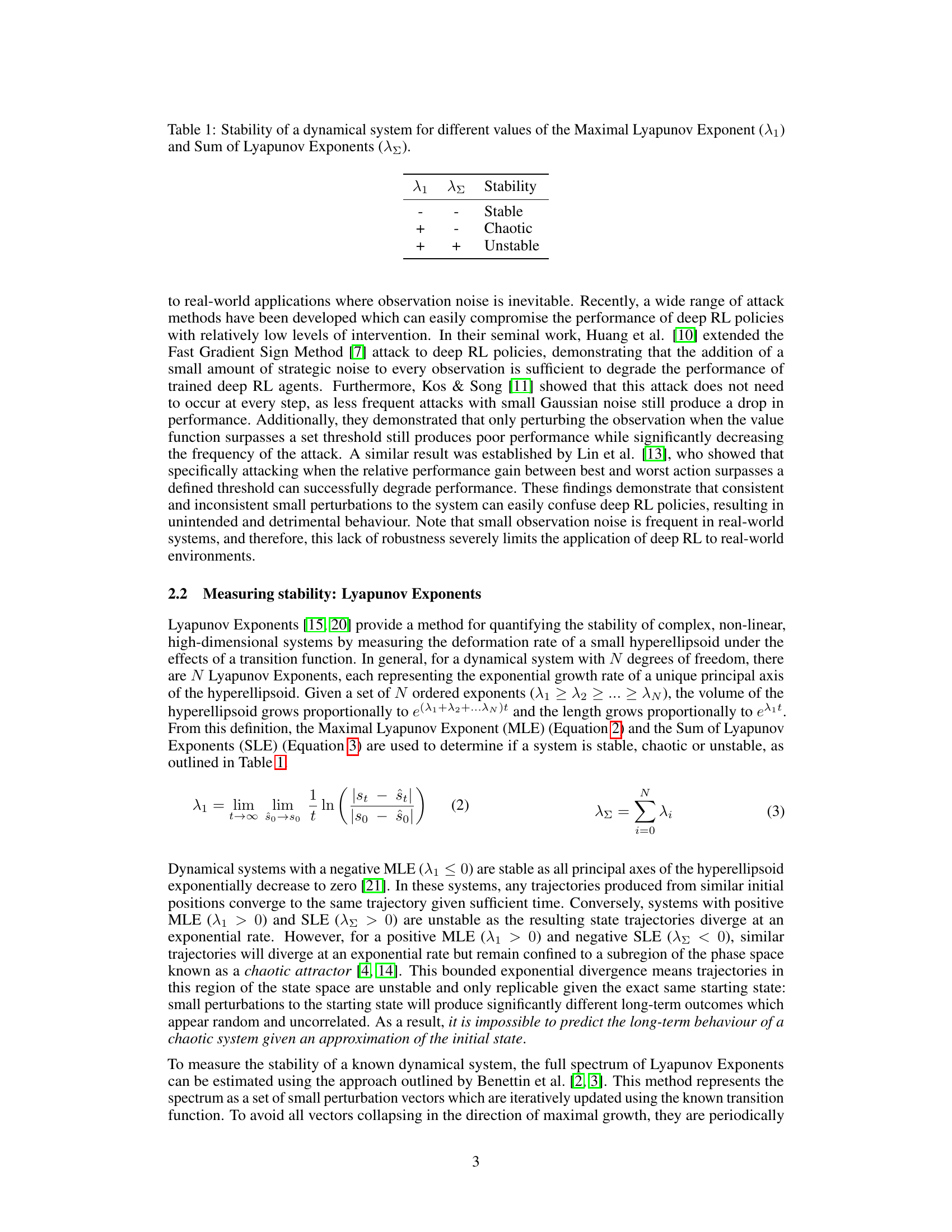
This table shows the stability of a dynamical system based on the signs of the maximal Lyapunov exponent (λ₁) and the sum of Lyapunov exponents (λε). A positive λ₁ indicates sensitive dependence on initial conditions, while a negative λ₁ suggests stability. The sign of λε further refines the classification: a positive λε indicates exponential divergence, while a negative λε implies convergence to an attractor (even if chaotic).

In-depth insights

#

Deep RL Robustness

#

Deep reinforcement learning (RL) agents demonstrate remarkable performance in simulated environments, yet their real-world applicability remains limited due to a lack of robustness. The core challenge lies in the sensitivity of deep RL policies to even minor perturbations in observations or states. Small amounts of noise, stemming from sensor inaccuracies or adversarial attacks, can drastically alter the agent’s behavior and lead to significant performance degradation. This fragility arises from the complex, often chaotic, dynamics inherent in the learned policies, characterized by high sensitivity to initial conditions and unpredictable long-term behavior. A key aspect of enhancing robustness involves understanding and mitigating this chaotic behavior. This necessitates techniques that promote stability and resilience against perturbations, such as incorporating Lyapunov Exponent regularization into the training process. This approach directly tackles the instability by constraining the rate of divergence of trajectories starting from nearby states. Future work should explore other methods for stabilizing RL agents, including more sophisticated control strategies and improved model architectures that inherently exhibit robustness against noisy or adversarial inputs. The pursuit of robust deep RL is crucial for its successful transition from simulation to the complexity and uncertainty of the real world.

MLE Regularization

#

The proposed Maximal Lyapunov Exponent (MLE) Regularization method addresses the instability and chaotic behavior often observed in deep reinforcement learning (RL) policies. By incorporating a regularisation term that estimates the local state divergence into the policy loss function, the method aims to constrain the MLE, thereby enhancing the robustness of the RL agent to perturbations and noise. This approach specifically targets chaotic state dynamics, where small changes in initial conditions can lead to significantly different long-term outcomes, impacting both the state trajectory and the cumulative reward. MLE regularization thus promotes the stability of the system, improving the reliability and predictability of its behavior in real-world scenarios where noisy observations or adversarial attacks are common. The method’s effectiveness is demonstrated experimentally, showing improvements in robustness to noise and enhanced performance, especially in higher-dimensional control tasks known for their sensitivity to initial conditions. This addresses a significant limitation of current deep RL approaches and contributes to the development of more reliable and safe RL agents for real-world applications.

Chaos in Deep RL

#

The concept of ‘Chaos in Deep RL’ explores the instability inherent in deep reinforcement learning (RL) agents. Deep RL agents, while achieving impressive results in simulations, often exhibit unpredictable behavior in real-world scenarios due to their sensitivity to small perturbations. This sensitivity stems from the complex, non-linear dynamics of the neural networks used in deep RL. Even slight variations in initial states or noisy observations can lead to significant divergences in agent trajectories and drastically different outcomes. This unpredictability poses a significant challenge for deploying deep RL in safety-critical applications. The presence of chaos manifests as a high sensitivity to initial conditions, creating a fractal return surface where small changes yield vastly different long-term outcomes. This directly impacts robustness and reliability, making it challenging to guarantee consistent performance. Addressing this challenge requires methods that enhance the stability of the learned policies, rendering them more resilient to noise and perturbations. This research area is crucial for bridging the gap between successful simulated performance and real-world applicability of deep RL.

Lyapunov Analysis

#

Lyapunov analysis, when applied to reinforcement learning (RL), offers a powerful lens for examining the stability and robustness of learned policies. By analyzing the Lyapunov exponents, which quantify the rate of divergence or convergence of nearby trajectories in the state space, we can assess the sensitivity of the RL agent’s behavior to small perturbations. A positive maximal Lyapunov exponent indicates chaotic dynamics, meaning that even tiny changes in the initial state can lead to drastically different long-term outcomes, hindering the reliable deployment of RL in real-world scenarios where noise and uncertainty are inevitable. Conversely, negative exponents signify stability and robustness. Therefore, Lyapunov analysis serves as a crucial tool for evaluating the generalization capabilities and reliability of RL agents, paving the way for developing more robust and predictable control policies. The integration of Lyapunov analysis into the design and training of RL agents can enable the development of more dependable control systems better suited for complex and uncertain environments.

Future Directions

#

Future research could explore several promising avenues. Improving the robustness of the MLE regularisation technique is crucial, potentially through adaptive methods that adjust the regularisation strength based on the observed system dynamics. Investigating different regularisation approaches beyond MLE is another important direction. For instance, exploring techniques that directly penalize chaotic behavior in the state-space or reward trajectories could yield significant improvements. Extending this work to more complex real-world environments, involving significant stochasticity or high dimensionality, is key to assessing the practical applicability and limitations of the proposed method. Finally, evaluating the efficacy of the proposed approach across different RL algorithms and architectural choices will help to understand its broad applicability and limitations. Developing more efficient methods for estimating Lyapunov exponents is important for scalable application to complex systems.

More visual insights

#

More on figures

This figure shows the total episode reward achieved by different reinforcement learning agents (SAC, TD3, DreamerV3, and a no-action baseline) across seven different DeepMind Control Suite environments. Each environment and agent combination was trained three times with different random seeds. The plot displays the average interquartile range of the total reward, along with a bootstrapped 95% confidence interval, based on 80 evaluation episodes per combination, each lasting 1000 steps. The results show the relative performance of the different algorithms on these diverse tasks.

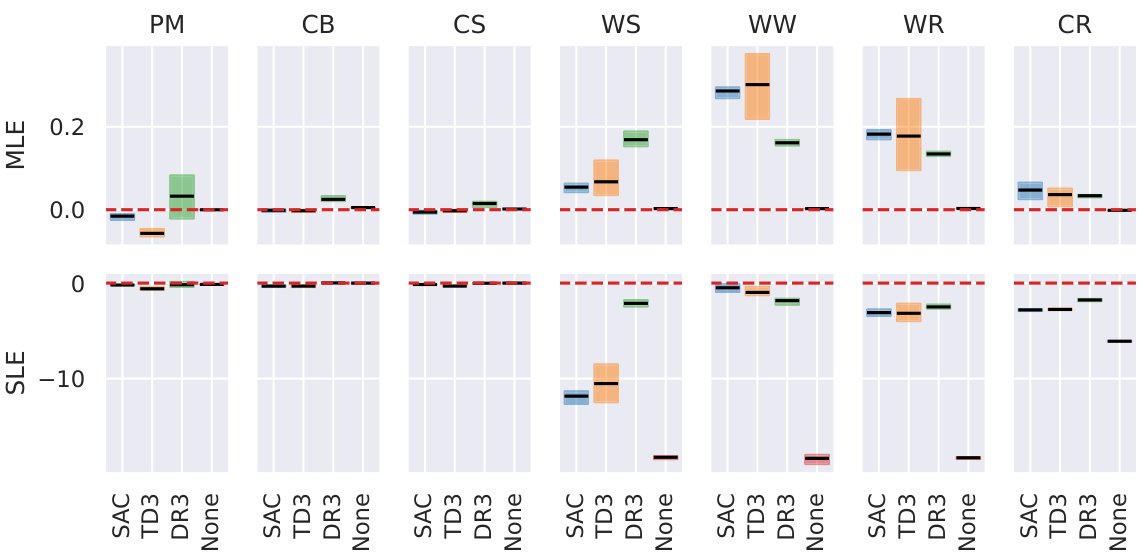
This figure displays the estimated Maximal Lyapunov Exponent (MLE) and Sum of Lyapunov Exponents (SLE) for seven DeepMind control suite environments controlled by four different reinforcement learning agents: SAC, TD3, DreamerV3, and a ‘None’ agent (taking no actions). The box plots show the interquartile range of MLE and SLE values across three independent training runs for each agent-environment combination, with the whiskers extending to the 95% confidence intervals. The results provide insights into the stability of different reinforcement learning agents across various environments, indicating which ones are more susceptible to chaotic dynamics.

This figure shows partial state trajectories for two different control tasks (Cartpole Balance and Walker Walk) when using the Dreamer V3 model. The trajectories are generated using nearly identical initial states (differing by only 10⁻⁴ units). The significant divergence of these trajectories highlights the chaotic nature of the control system. Small initial differences quickly lead to vastly different system behaviors.

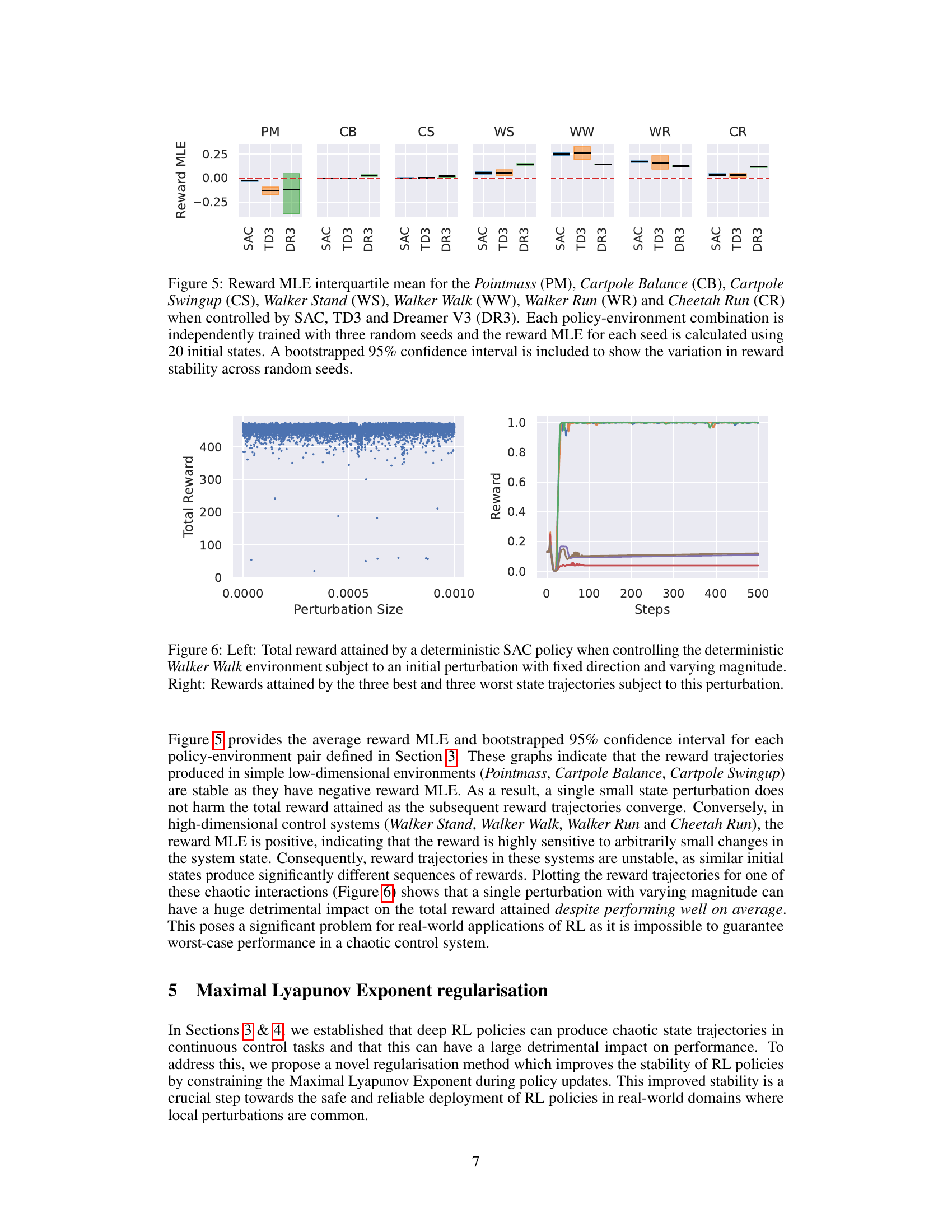
The figure shows the Maximal Lyapunov Exponent (MLE) of the reward for different control tasks (Pointmass, Cartpole Balance, Cartpole Swingup, Walker Stand, Walker Walk, Walker Run, and Cheetah Run) when controlled by three different reinforcement learning algorithms (SAC, TD3, and DreamerV3). Each bar represents the interquartile range of the reward MLE across three independent training runs, and the whiskers show the 95% confidence intervals. A red dashed line is drawn at MLE = 0 to show the transition between stable (negative MLE) and chaotic (positive MLE) reward dynamics. The figure shows that the reward dynamics are stable for simple low-dimensional tasks but become chaotic for higher-dimensional tasks, regardless of the RL algorithm used.

The left panel shows how the total reward changes with different perturbation sizes when a deterministic SAC policy controls the Walker Walk environment. The right panel displays the reward trajectories for the three best-performing and three worst-performing instances, highlighting the significant variability in outcomes due to the chaotic nature of the system.

This figure displays the total reward obtained by four different reinforcement learning algorithms (SAC, TD3, DR3, and MLE DR3) across six different control tasks from the DeepMind Control Suite. Each algorithm was trained without noise and then tested with varying levels of Gaussian observation noise (σ). The plot shows the average total reward and its 95% confidence interval across multiple trials for each algorithm and task.

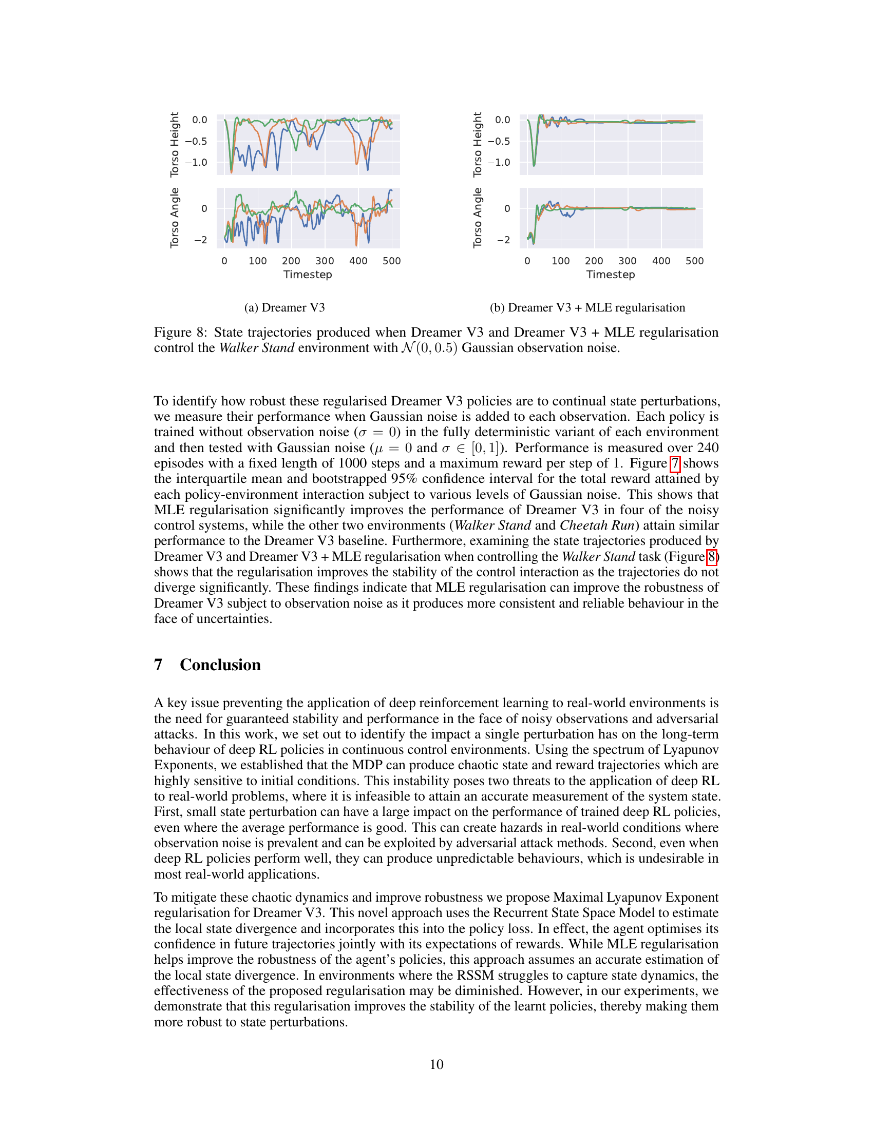
This figure shows the torso angle and torso height trajectories produced by Dreamer V3 and the proposed Dreamer V3 + MLE regularisation method when controlling the Walker Stand environment. The trajectories start from slightly different initial states and are subject to N(0, 0.5) Gaussian observation noise, which introduces continuous state perturbations. The plot visually demonstrates the effect of MLE regularisation on stabilizing the state trajectories and reducing the sensitivity to noise. The Dreamer V3 trajectories show significant divergence, while the Dreamer V3 + MLE regularisation trajectories exhibit much greater stability and convergence.

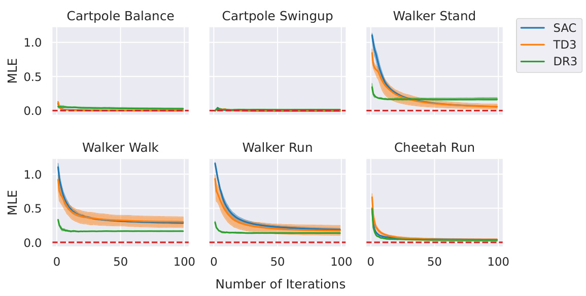
This figure shows the estimated Maximal Lyapunov Exponent (MLE) for different environments from the DeepMind Control Suite, controlled by three different reinforcement learning algorithms (SAC, TD3, and Dreamer V3). The x-axis represents the number of iterations used to calculate the MLE, and the y-axis represents the MLE value. The shaded area around each line represents the 95% confidence interval. The plot demonstrates that the MLE generally converges after around 100 iterations for all algorithms and environments.

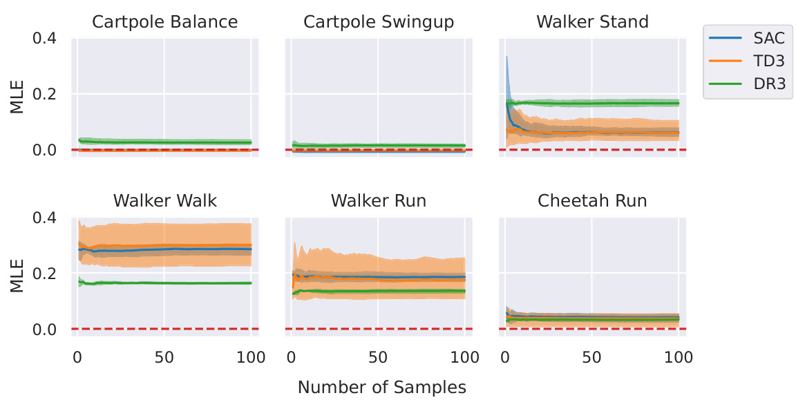
This figure shows the estimated Maximal Lyapunov Exponent (MLE) for different DeepMind Control Suite environments controlled by three different reinforcement learning algorithms (SAC, TD3, and Dreamer V3). It investigates how the number of initial samples used to calculate the MLE affects the convergence of the MLE estimation. The results show MLE convergence is achieved with 20 initial samples.

More on tables

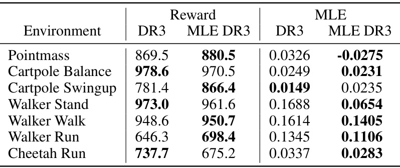
This table presents the average total reward and Maximal Lyapunov Exponent (MLE) achieved by two different models, Dreamer V3 (DR3) and a modified version with MLE regularization (MLE DR3), across seven different control environments from the DeepMind Control Suite. Each environment was tested with three separate random seeds to ensure robustness of the results, and hyperparameters used were consistent across all tests (Appendix A.2). The data highlights the impact of MLE regularization on both reward performance and system stability, indicated by the MLE values. A lower MLE value implies greater stability.

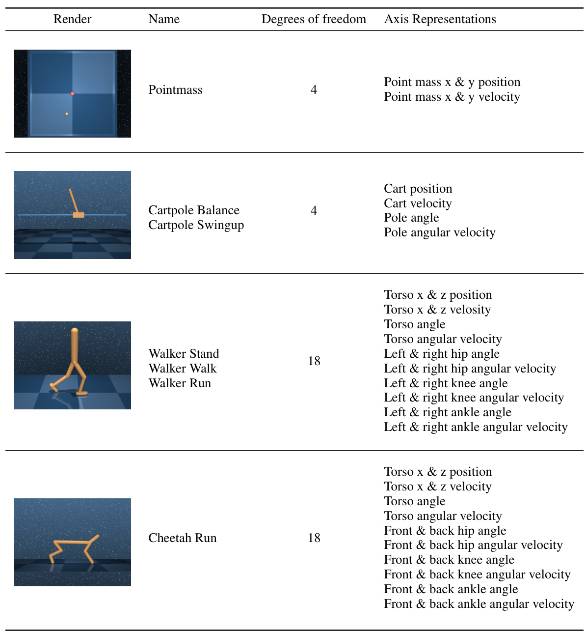
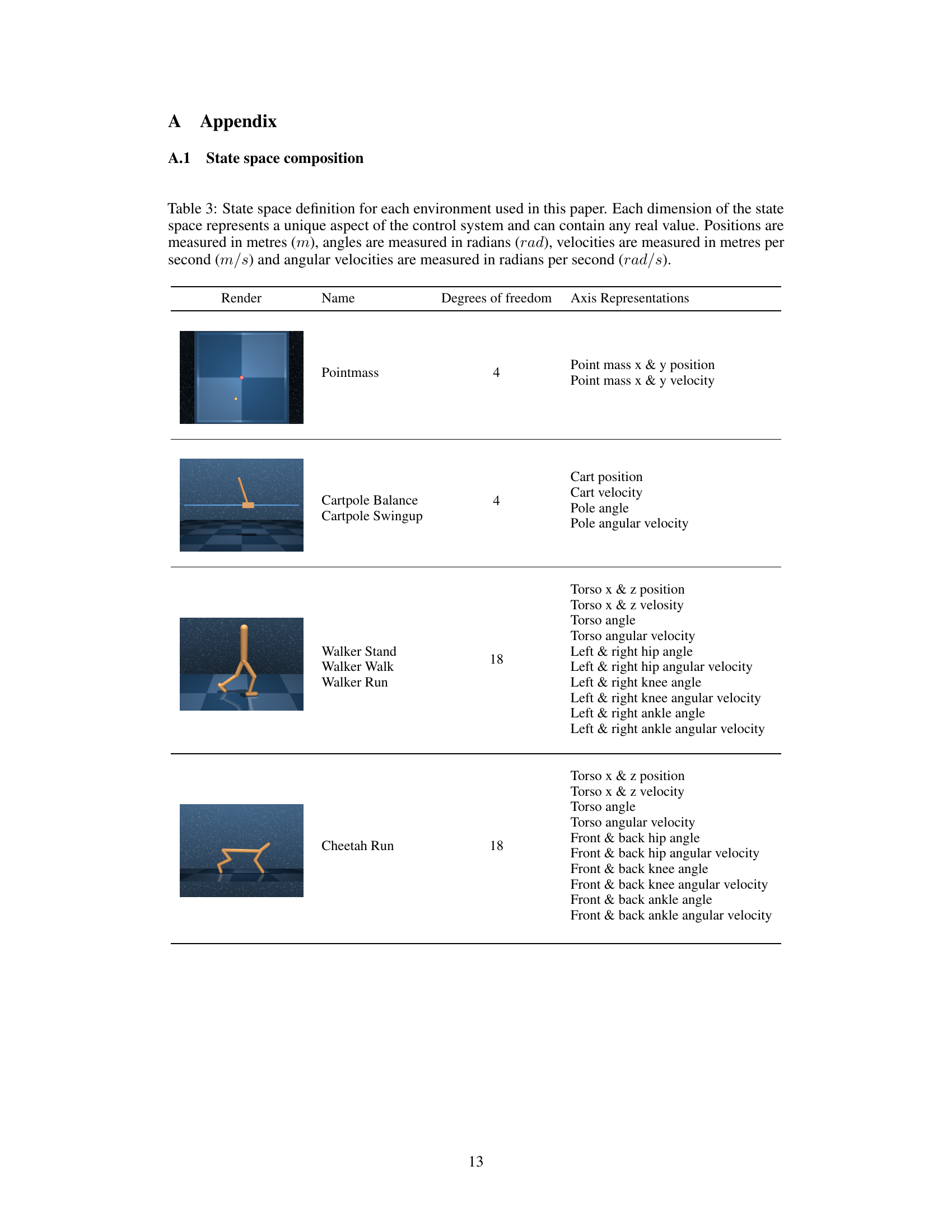
This table details the state space composition for each of the seven DeepMind control suite environments used in the paper. For each environment, it lists the number of degrees of freedom and specifies the physical quantities represented by each dimension of the state space (position, angle, velocity, angular velocity), including their units of measurement.

This table presents the hyperparameters used for training three different reinforcement learning algorithms: Soft Actor-Critic (SAC), Twin Delayed Deep Deterministic policy gradients (TD3), and Dreamer V3. For each algorithm, the table lists the values used for various parameters, including environment steps, buffer size, parallel environments, update period, updates per step, discount factor, learning rate, batch size, Polyak update coefficient, network activation function, network depth, and network width.

This table lists the hyperparameters used for training three different reinforcement learning algorithms: Soft Actor-Critic (SAC), Twin Delayed Deep Deterministic policy gradients (TD3), and Dreamer V3. For each algorithm, it shows the values used for parameters such as environment steps, buffer size, parallel environments, update period, updates per step, discount factor, learning rate, batch size, polyak update coefficient (for SAC and TD3), network activation function, network depth, and network width. Dreamer V3 also includes parameters specific to its model-based approach such as RSSM batch length and imagination horizon. These hyperparameters were used in the experiments described in the paper to train the RL agents.

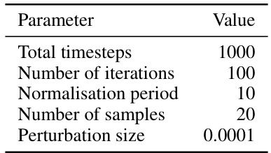
This table shows the hyperparameters used to compute the Lyapunov exponents, which are key to characterizing the stability and chaos in the dynamical systems studied in the paper. These parameters control aspects of the numerical calculation process, such as the length of trajectories, the frequency of orthonormalization, and the magnitude of initial state perturbations.

Full paper

#