↗ OpenReview ↗ NeurIPS Homepage ↗ Hugging Face ↗ Chat
TL;DR#
Disentangled Representation Learning (DRL) holds immense potential for AI, but its application to real images is hindered by correlated generative factors, limited resolution, and scarce ground-truth labels. This paper tackles this challenge by exploring the use of synthetic data to learn general-purpose disentangled representations that can be effectively transferred to real data. It investigates the impact of fine-tuning and assesses which properties of disentanglement are preserved after the transfer.
The study introduces a new, interpretable intervention-based metric, OMES, to quantitatively assess the quality of disentangled representations. Extensive experiments demonstrate the feasibility and effectiveness of transferring disentangled representations from synthetic to real images, addressing the limitations of existing DRL approaches. The results showcase the benefits of this transfer, bridging the gap between the controlled environment of synthetic data and complex, real-world scenarios.
Key Takeaways#
Why does it matter?#
This paper is crucial for researchers in disentangled representation learning and domain adaptation. It introduces a novel metric for evaluating disentanglement, offers a practical methodology for transferring disentangled representations from synthetic to real data, and demonstrates its effectiveness. This work directly addresses the challenge of applying DRL to real-world scenarios, opening new avenues for research in robust and generalizable AI.
Visual Insights#

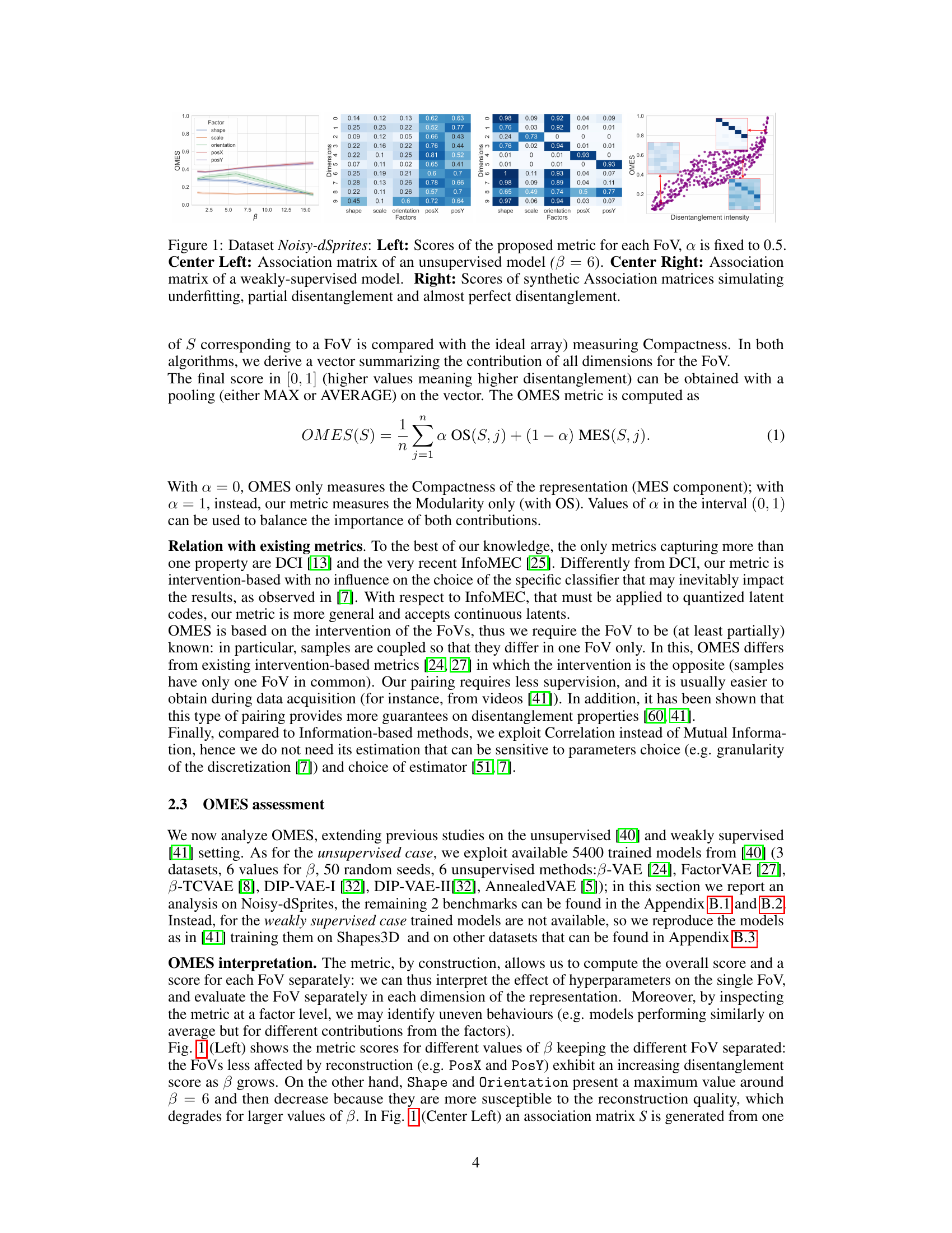
This figure presents an analysis of the OMES metric on the Noisy-dSprites dataset. The left panel shows the OMES scores for each factor of variation (FoV) with a fixed parameter alpha (α) of 0.5. The center-left and center-right panels display association matrices representing unsupervised and weakly-supervised models, respectively. The right panel visualizes OMES scores from synthetic association matrices representing varying levels of disentanglement, ranging from underfitting to near-perfect disentanglement. This figure demonstrates the metric’s ability to assess the quality of disentanglement across different models and conditions.

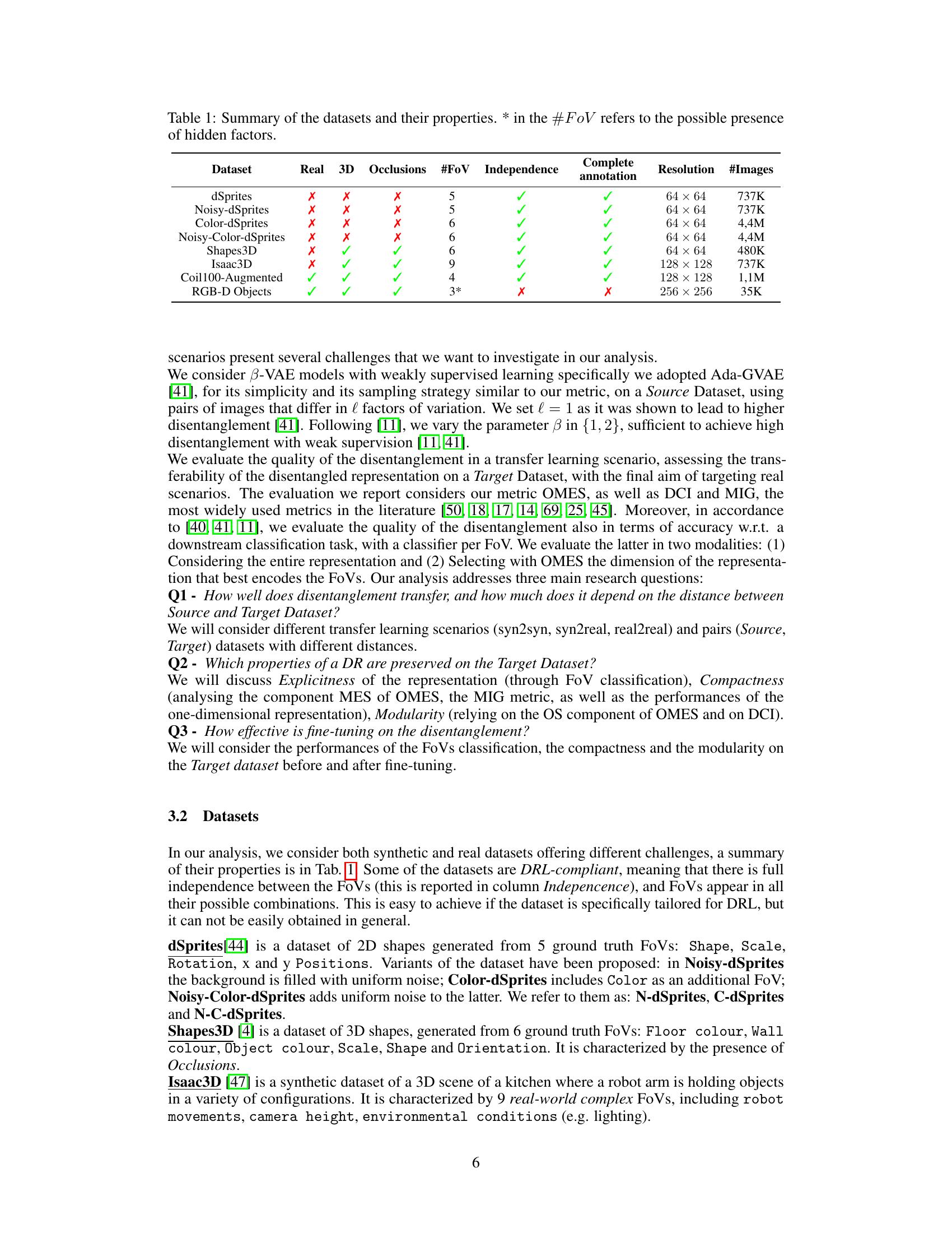
This table summarizes the properties of several datasets used in the paper’s experiments. For each dataset, it indicates whether it contains real or synthetic images, whether it involves 3D or 2D objects, the presence of occlusions, the number of factors of variation (FoVs), whether the FoVs are independent, and whether there is complete annotation of the factors. It also specifies the resolution and the number of images in each dataset. The asterisk (*) next to #FoV denotes the possibility of hidden factors.
In-depth insights#
Disentanglement Metrics#
Disentanglement metrics are crucial for evaluating the quality of learned representations in disentangled representation learning (DRL). A good disentanglement metric should capture the degree to which the learned factors of variation are truly independent and interpretable. However, defining and measuring disentanglement remains a challenge, with various metrics proposed, each with its strengths and weaknesses. Some metrics rely on the mutual information between latent variables and factors, while others employ intervention-based approaches or rely on the performance of downstream tasks. The choice of metric can significantly impact the conclusions drawn about a DRL model’s performance. An ideal metric would be both robust and highly sensitive to different aspects of disentanglement, including the level of independence, completeness, and explicitness of the learned factors. Furthermore, the interpretability and computational efficiency of the metric are important practical considerations. The development of better metrics is an active area of research; it directly impacts the progress and evaluation of DRL methods.
DR Transfer Approach#
The core of this research lies in its novel DR transfer approach, designed to bridge the gap between synthetic and real-world image data. The methodology is weakly supervised, leveraging labeled synthetic data to learn disentangled representations, then transferring these to unlabeled real data. This process avoids the high cost and infeasibility of labeling real datasets for each factor of variation. The study focuses on the transferability of disentanglement, exploring the effects of fine-tuning and analyzing which properties of disentanglement (modularity, compactness, and explicitness) are preserved. A key contribution is the introduction of a novel, interpretable metric to quantify disentanglement quality, supplementing existing measures. The results demonstrate that some level of disentanglement transfer is achievable, highlighting the practical potential of leveraging synthetic data for general-purpose disentangled representation learning.
Synthetic-Real Gap#
The ‘Synthetic-Real Gap’ in disentangled representation learning highlights the challenge of transferring models trained on idealized synthetic data to complex real-world scenarios. Synthetic datasets offer controlled environments with readily available ground truth labels, facilitating disentanglement learning. However, real images present significant challenges, including correlated generative factors, resolution differences, and limited access to accurate ground truth labels. This gap limits the practical applicability of DRL models. Bridging this gap requires addressing these factors, such as developing robust methods for handling noisy or incomplete real data and exploring techniques that leverage synthetic data to learn general-purpose representations that generalize well. Fine-tuning strategies are crucial to adapt representations from a controlled synthetic domain to real data. A key focus should be on the properties of disentanglement preserved after transfer, as well as the development of new metrics that assess the quality of the transferred representation in real-world settings.
Fine-tuning Effects#
Fine-tuning’s impact on disentangled representations after transfer from synthetic to real data is a crucial aspect. Positive effects are expected, improving the model’s ability to generalize and adapt to the complexities of real-world images. However, the degree of improvement is likely to vary depending on factors such as the similarity between the source and target data domains, the quality of the initial disentanglement, and the fine-tuning process itself. Overfitting is a potential risk, where the model becomes too specialized to the target dataset and loses its generalization ability. Careful monitoring of metrics like classification accuracy and disentanglement scores during fine-tuning is essential to prevent overfitting and to determine the optimal level of fine-tuning. The balance between enhanced performance and preservation of initial disentanglement must be considered. Analyzing the specific factors that benefit most from fine-tuning could offer insights into the transferability of disentanglement and the model’s capacity for domain adaptation.
Future Research#
The paper concludes by outlining several promising avenues for future work. Extending the disentanglement transfer methodology to other VAE-based approaches and beyond is crucial for broader applicability. Investigating the impact of latent space dimensionality and varying degrees of supervision during both initial training and fine-tuning warrants further investigation. Applying this methodology to more complex real-world datasets, particularly those with hidden or unannotated factors of variation, presents a significant challenge. The need to develop quantitative methods for assessing the semantic similarity between source and target datasets is also highlighted. Finally, the authors suggest exploring specific application domains, such as biomedical image analysis or action recognition, to ascertain the practical efficacy of disentanglement transfer in challenging scenarios.
More visual insights#
More on figures

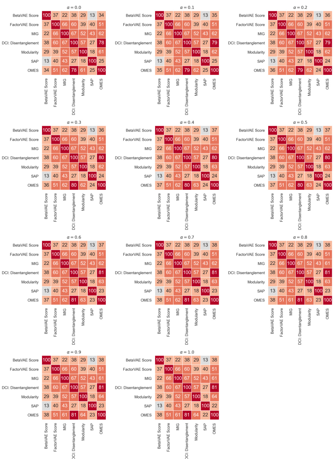
This figure presents three plots that analyze the relationship between disentanglement metrics and model performance. The left plot shows the rank correlation between different disentanglement metrics (including the proposed OMES metric) when models are trained on the Noisy-dSprites dataset. The center plot displays the distribution of these same metrics for models trained on the same dataset. Finally, the right plot illustrates the Spearman rank correlation between ELBO, reconstruction loss, and classification accuracy (using GBT and MLP classifiers) with the disentanglement metrics. All analyses in the figure use the OMES metric with α=0.5, indicating a balanced consideration of both Modularity and Compactness.

This figure shows boxplots of the OMES scores for seven different association matrices. The first three matrices (I-III) are simulated with varying degrees of overlap and multiple encoding, while the last four matrices (IV-VII) are obtained from real and synthetic datasets using weakly supervised and unsupervised methods. The figure demonstrates the ability of OMES to distinguish between different levels of disentanglement.

This figure presents an analysis of the OMES metric on the Noisy-dSprites dataset. The left panel shows the scores for each factor of variation (FoV) with alpha fixed at 0.5. The center-left panel displays the association matrix for an unsupervised model with beta=6, while the center-right panel shows the matrix for a weakly supervised model. The right panel illustrates OMES scores for synthetic association matrices representing underfitting, partial disentanglement, and near-perfect disentanglement.

This figure displays boxplots showing the distribution of OMES scores for seven different association matrices. Three matrices represent simulated scenarios with varying degrees of overlap and multiple encoding, while the remaining four matrices are derived from real-world datasets with weak supervision or unsupervised learning. The boxplots help to visualize how the OMES score, which measures the quality of disentanglement, varies across these different scenarios and models.
This figure presents the results of the proposed OMES metric for evaluating disentanglement. The left panel shows OMES scores for each factor of variation (FoV) in the Noisy-dSprites dataset. The center panels display association matrices illustrating the relationships between dimensions of a disentangled representation and the FoVs for both unsupervised and weakly-supervised models. The right panel shows how OMES scores change with varying degrees of disentanglement in simulated data, ranging from underfitting to almost perfect disentanglement.

This figure shows the evaluation of the OMES metric on the Noisy-dSprites dataset. The left panel displays the scores of the proposed metric for each factor of variation (FoV), with α fixed at 0.5. The center-left panel shows the association matrix of an unsupervised model (β=6). The center-right panel displays the association matrix for a weakly supervised model. Finally, the right panel illustrates the scores obtained from synthetic association matrices, which simulate different levels of disentanglement: underfitting, partial disentanglement, and near-perfect disentanglement. These visual representations help assess how well the OMES metric captures the degree of disentanglement in different scenarios.
This figure presents an evaluation of the OMES metric on the Noisy-dSprites dataset. The left panel shows the OMES scores for each factor of variation (FoV) with alpha fixed at 0.5, demonstrating how the metric scores different aspects of disentanglement. The center-left panel displays the association matrix for an unsupervised model, while the center-right panel presents the association matrix for a weakly supervised model. Finally, the right panel illustrates the scores obtained from synthetic association matrices that simulate various degrees of disentanglement (underfitting, partial disentanglement, and almost perfect disentanglement). This visualization helps illustrate the metric’s ability to capture the degree of disentanglement in different models and its sensitivity to varying levels of disentanglement intensity.

This figure shows the evaluation of the proposed OMES metric on the Noisy-dSprites dataset. The left panel displays OMES scores for each factor of variation (FoV) with the hyperparameter alpha set to 0.5. The center-left and center-right panels present association matrices, visualizing the relationship between latent dimensions and FoVs, for an unsupervised and a weakly supervised model, respectively. Finally, the right panel illustrates how OMES scores change based on synthetic association matrices that represent underfitting, partial disentanglement, and near-perfect disentanglement.

This figure presents an analysis of the OMES metric applied to the Noisy-dSprites dataset. The left panel shows the scores for each factor of variation (FoV), demonstrating how well the metric captures disentanglement for different factors. The center-left and center-right panels illustrate association matrices for unsupervised and weakly supervised models, respectively, visualizing how dimensions of the representation relate to the FoVs. The right panel showcases the OMES scores for synthetic association matrices, illustrating the metric’s ability to discriminate between different levels of disentanglement, from underfitting to near-perfect disentanglement.
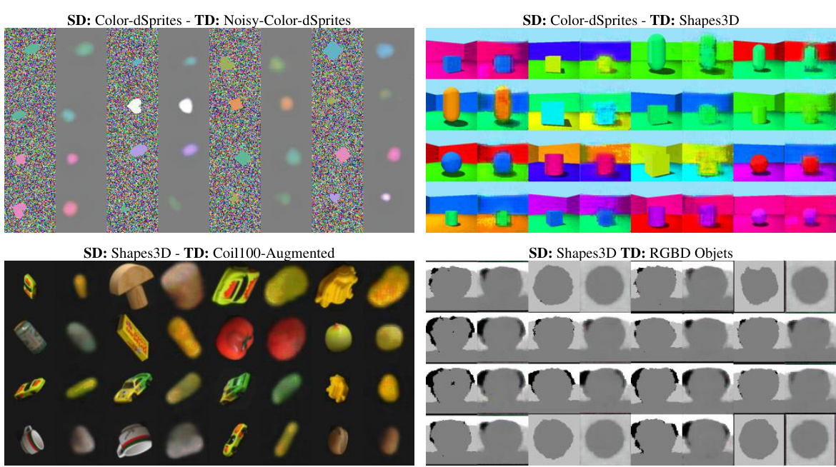
This figure shows some reconstruction examples obtained by fine-tuned models of different source and target datasets. The fine-tuning process involves training a Variational Autoencoder (VAE) model on a source dataset, then fine-tuning it on a target dataset. The figure demonstrates that the fine-tuned models can reconstruct images from target datasets, even when the source and target datasets are different, indicating a degree of successful transfer learning.

This figure displays reconstruction samples from fine-tuned models, trained initially on various source datasets (SD) and subsequently fine-tuned on different target datasets (TD). The image pairs demonstrate the model’s ability to generate reasonable reconstructions even after transferring the representation from significantly different datasets. The visual quality of the reconstructions helps to assess the effectiveness of the disentangled representation transfer.

This figure presents an evaluation of the proposed OMES metric and its ability to capture different levels of disentanglement. The leftmost panel shows OMES scores for each factor of variation (FoV) in the Noisy-dSprites dataset, with alpha fixed at 0.5. The center panels display association matrices illustrating the relationships between dimensions of the latent representation and the FoVs for both unsupervised and weakly-supervised models. The rightmost panel demonstrates the OMES scores for synthetic association matrices designed to represent underfitting, partial disentanglement, and near-perfect disentanglement scenarios. This visualization helps to demonstrate the metric’s sensitivity and interpretability in assessing various degrees of disentanglement.

This figure presents an analysis of the OMES (Overlap Multiple Encoding Scores) metric on the Noisy-dSprites dataset. The left panel shows the scores for each factor of variation (FoV) with the parameter ‘a’ set to 0.5. The center-left panel displays the association matrix for an unsupervised model with beta = 6, visualizing the relationships between latent dimensions and FoVs. The center-right panel shows the association matrix for a weakly-supervised model. Finally, the right panel illustrates OMES scores from synthetically generated association matrices representing varying levels of disentanglement (underfitting, partial disentanglement, and almost perfect disentanglement). This comprehensive visualization demonstrates the metric’s ability to capture different degrees of disentanglement.
More on tables

This table summarizes the characteristics of eight datasets used in the paper’s experiments. For each dataset, it indicates whether it contains real or synthetic images (Real), whether the images are 3D or 2D (3D), whether occlusions are present (Occlusions), the number of factors of variation (FoV), whether the FoVs are independent, if complete annotations are available, the resolution of images, and the number of images in the dataset. The asterisk (*) in the #FoV column indicates the potential presence of hidden or unannotated factors. This table is crucial for understanding the diversity and complexity of the data used in evaluating the proposed disentangled representation transfer methodology.

This table presents a quantitative analysis of transferring disentangled representations within the dSprites family of datasets. It shows the average classification accuracy (using Gradient Boosted Trees) before and after fine-tuning, comparing performance using the full representation versus a pruned representation (selected based on the OMES metric). The table also includes measures of disentanglement (MES, OS, DCI, MIG).

This table presents a quantitative analysis of transferring disentangled representations within the dSprites family of datasets. It shows the average classification accuracy (using Gradient Boosted Trees) for various factors of variation (FoVs), both before and after applying a dimensionality reduction technique guided by the OMES metric (Pruned). The results are broken down by source and target datasets, showcasing the impact of the transfer on different aspects of disentanglement. Finally, it includes a comparison using disentanglement metrics like MES, OS, DCI, and MIG to evaluate the overall quality of the disentangled representations after transfer.

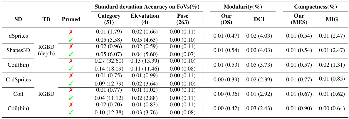
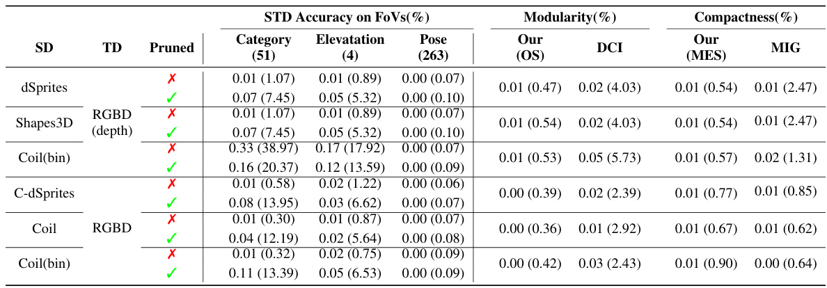
This table presents the results of transferring disentangled representations from different source datasets to the Coil-100 dataset and its variants. It shows the average classification accuracy for different factors of variation (FoVs), along with disentanglement metrics (Modularity and Compactness) before and after fine-tuning. The ‘Pruned’ column indicates whether only the most relevant dimension according to the OMES metric was used for classification. It helps to understand the performance of the transfer learning and the preservation of disentanglement properties in the target domain.

This table presents a quantitative evaluation of transferring disentangled representations within the dSprites family of datasets. It shows the average classification accuracy using Gradient Boosted Trees (GBT) for various source-target dataset pairs, both with the full representation and a ‘pruned’ representation (using only the most informative dimension). Disentanglement is evaluated using MES, OS, DCI, and MIG metrics.

This table compares various metrics used for evaluating disentanglement in representation learning. It shows whether each metric is based on intervention, information theory, or prediction; the type of classifier (if any) used; the number of classifiers; and the disentanglement property (modularity or compactness) measured by each metric. The table provides a useful overview of the existing approaches to evaluating disentanglement, highlighting their strengths and weaknesses.

This table summarizes several metrics used to evaluate disentanglement in representation learning. It compares various approaches based on whether they are intervention-based, information-based, or predictor-based. The table also specifies the classifier used (if any), the number of classifiers, and the disentanglement property each metric measures (Modularity, Compactness, or Explicitness). This allows for a comparison of different methods and their strengths in evaluating specific aspects of disentanglement.

This table presents the average classification accuracy of a Gradient Boosted Trees (GBT) classifier on the Isaac3D dataset. The classifier is trained using the disentangled representations learned from the Shapes3D dataset. The table shows the performance both before and after fine-tuning the model on the Isaac3D dataset. The results are broken down by individual Factors of Variation (FoVs) in the Isaac3D dataset, and also shows an overall accuracy across all FoVs. The ‘Pruned’ row indicates whether a single dimension (the one with strongest OMES score for the FoV) was used in the classification or the entire representation was used.

This table shows the compactness and modularity scores for the same models used in Table 9. The compactness and modularity are evaluated using the OMES metric (both OS and MES components) and also using DCI and MIG metrics. The results show the values before and after fine-tuning, indicating the impact of the fine-tuning process on these two important properties of disentangled representations.

This table presents a quantitative evaluation of how well disentangled representations transfer between different datasets in the dSprites family. It shows the average classification accuracy (using Gradient Boosted Trees) for various factors of variation (FoVs), both using the full representation and a pruned version (selected using the OMES metric). It also compares disentanglement using different metrics (MES, OS, DCI, MIG). The source and target datasets are specified, and the improvements from fine-tuning are indicated.

This table presents a quantitative evaluation of the transfer learning experiments using the dSprites dataset family. It shows the average classification accuracy obtained by using Gradient Boosted Trees (GBT) on both the full and pruned (one-dimensional) representations. The table compares results for different Source and Target datasets, indicating which FoVs (Factors of Variation) were used. The final columns provide a comparison of various disentanglement metrics (including the proposed OMES metric).

This table presents a quantitative evaluation of transferring disentangled representations using the dSprites dataset family. It shows the average classification accuracy (using Gradient Boosted Trees) on various target datasets, comparing results obtained using the full representation versus a pruned (single-dimension) representation. The table also includes a comparison of disentanglement metrics (MES, OS, DCI, MIG) to assess the quality of the transferred representation. The source dataset varies across different rows, while the target datasets (and the use of the pruned representation) are systematically varied to explore the impact of this transfer.

This table presents a quantitative analysis of transferred disentangled models using the dSprites family of datasets. It shows the average classification accuracy (using Gradient Boosted Trees) for different Source and Target datasets, both with the full representation and a pruned representation (using only the most relevant dimension as determined by OMES). The table compares the performance before and after fine-tuning, and also includes a comparison of disentanglement metrics like MES (Multiple Encoding Score), OS (Overlap Score), DCI (Disentanglement), and MIG (Mutual Information Gap).

This table presents a quantitative analysis of transferring disentangled representations within the dSprites family of datasets. It shows the average classification accuracy (using Gradient Boosted Trees) on different factors of variation (FoVs), both using the full representation and a pruned representation (selected using the OMES metric). The table also includes disentanglement scores (MES, OS, DCI, MIG) to evaluate the quality of the transferred representation. The comparison is made for various source-target dataset pairs, allowing assessment of transfer performance across different levels of similarity between the source and target data.

This table summarizes the characteristics of several datasets used in the paper’s experiments. It lists whether each dataset is real or synthetic, if it contains 3D information or occlusions, the number of factors of variation (#FoV) it contains, whether these factors are independent or correlated, if complete annotations are available for all FoVs, and the resolution and number of images in each dataset. The asterisk (*) next to #FoV indicates that hidden factors might exist in that dataset.

This table summarizes the characteristics of several datasets used in the paper’s experiments. It shows whether each dataset is real or synthetic, if it involves 3D data or occlusions, the number of factors of variation (FoVs), whether the FoVs are independent, if complete annotations are available, the image resolution, and the total number of images. The asterisk (*) indicates that there might be hidden factors in the dataset.
This table summarizes the characteristics of several datasets used in the paper’s experiments. For each dataset, it indicates whether it consists of real or synthetic images, if it includes 3D information, if occlusions are present, the number of factors of variation (FoVs), whether the FoVs are independent, whether complete annotations are available, the image resolution, and the number of images.

This table summarizes the characteristics of several datasets used in the paper’s experiments. It shows whether each dataset is real or synthetic, whether it involves 3D objects or occlusions, the number of factors of variation (#FoV), whether the factors are independent, whether there is complete annotation of the FoVs, the image resolution, and the number of images. The asterisk (*) next to the #FoV indicates the potential presence of hidden factors. The table helps to understand the diversity of data used in evaluating the proposed method for transferring disentangled representations, highlighting the differences in complexity and supervision.

This table presents a quantitative evaluation of transferred disentangled models, focusing on the dSprites family of datasets. It shows the average classification accuracy achieved using Gradient Boosted Trees (GBT) on both the full and pruned latent representations. The table compares results across different source and target datasets, analyzing the impact of transferring a disentangled representation from one dataset to another. The final columns provide a comparison using different disentanglement metrics (MES, OS, DCI, MIG).

This table presents a quantitative evaluation of transferring disentangled models within the dSprites family of datasets. It shows the average classification accuracy using Gradient Boosted Trees (GBTs) on both the full and pruned representations (where the representation is reduced to only the most informative dimension for each factor of variation). The results are presented for various Source-Target dataset pairs, illustrating how well disentanglement transfers in different scenarios. It also includes a comparison of disentanglement metrics like MES (Multiple Encoding Score), OS (Overlap Score), DCI (Disentanglement), and MIG (Mutual Information Gap) to assess the quality of the transferred representations.
This table summarizes the characteristics of several datasets used in the paper’s experiments. It shows whether each dataset is real or synthetic, whether it includes 3D information or occlusions, the number of factors of variation (#FoV), whether the factors are independent, whether complete annotations are available, the resolution of the images, and the number of images in each dataset. The asterisk (*) indicates that the dataset may have hidden factors not explicitly identified.
Full paper#

