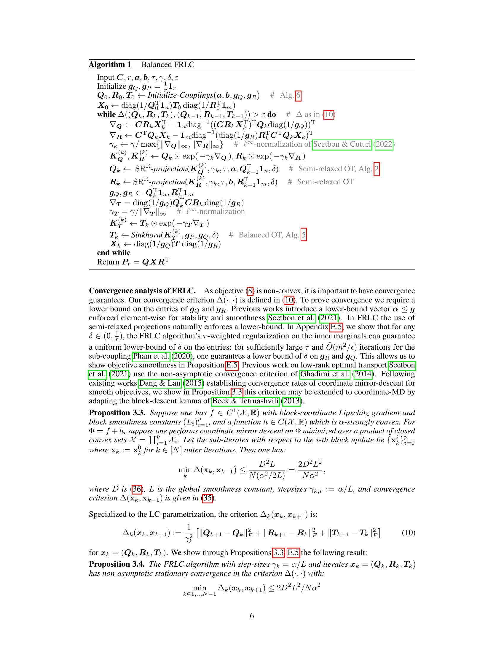
↗ OpenReview ↗ NeurIPS Homepage ↗ Chat
TL;DR#
Optimal transport (OT) is a powerful tool for comparing probability distributions, but its quadratic scaling with dataset size limits its applicability to massive datasets. Existing low-rank methods aim to address this issue by factoring the transport plan, but they often lack flexibility and interpretability. The computational complexity of these methods also poses a challenge.
This paper introduces Factor Relaxation with Latent Coupling (FRLC), a novel algorithm that leverages a latent coupling factorization to compute low-rank transport plans. FRLC’s key advantages include decoupling the optimization into three smaller OT problems, enhanced flexibility to handle various OT objectives and marginal constraints, and improved interpretability through the latent coupling. The researchers demonstrate FRLC’s superior performance on diverse applications, highlighting its efficiency and ability to reveal meaningful insights from complex datasets.
Key Takeaways#
Why does it matter?#
This paper is crucial for researchers working with large datasets and complex comparisons. It introduces a novel, interpretable method for low-rank optimal transport, significantly improving efficiency and scalability while maintaining accuracy. This opens avenues for broader applications in various fields, especially where large datasets are commonplace.
Visual Insights#
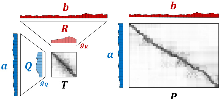
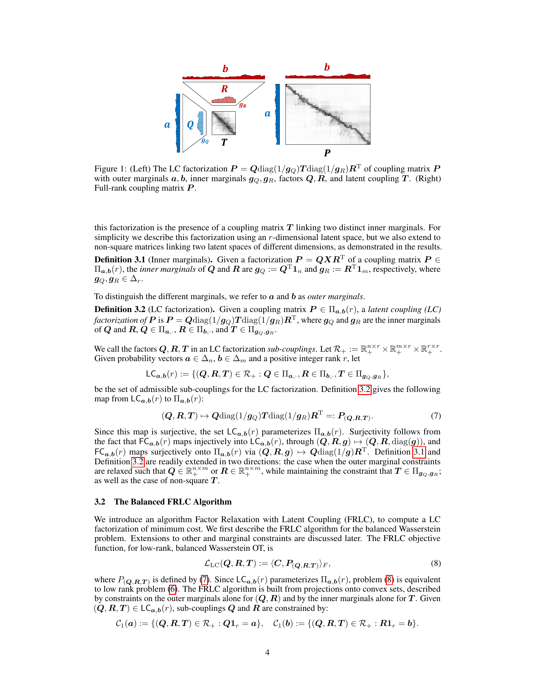
This figure shows a comparison between the low-rank latent coupling factorization of the optimal transport plan (left) and the full rank optimal transport plan (right). The low-rank factorization decomposes the coupling matrix P into three smaller matrices: Q, R, and T. Q and R are sub-couplings with inner marginals gQ and gR respectively. T is a latent coupling matrix that links the inner marginals. This decomposition allows for efficient computation of the optimal transport plan, especially for high-dimensional data.
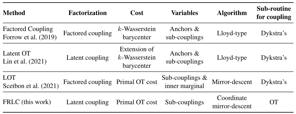
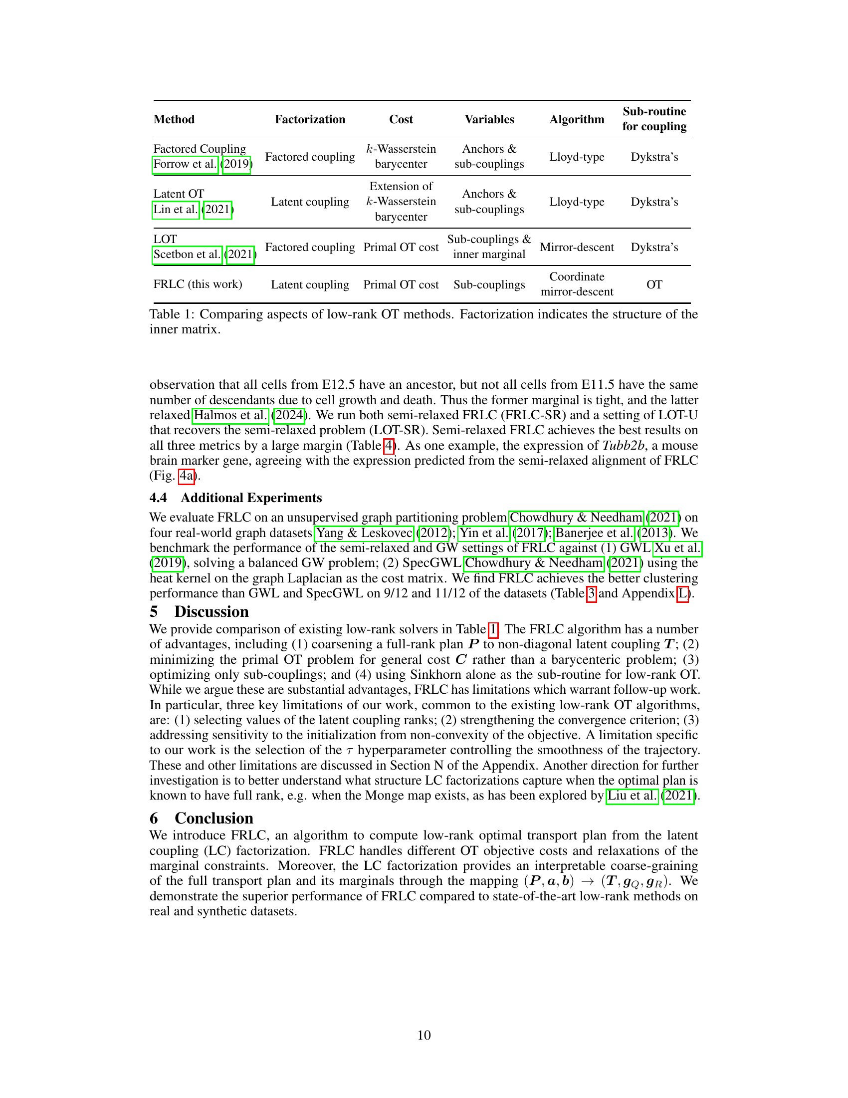
This table compares several low-rank optimal transport methods, focusing on their factorization approach (how the transport plan is factorized), the cost function they optimize, the variables involved in the optimization, the algorithm used for optimization, and the specific sub-routine used for handling the coupling matrices. The table highlights the differences in the mathematical formulations and optimization strategies employed by various low-rank optimal transport methods, illustrating their diverse approaches to solving the low-rank OT problem.
In-depth insights#
Low-Rank OT#
Low-rank Optimal Transport (OT) methods address the computational challenges of standard OT, which scales quadratically with dataset size. Low-rank OT approximates the dense coupling matrix P with a lower-rank factorization, significantly reducing memory and computational demands. This is crucial for large-scale applications. Several factorization approaches exist, each with trade-offs. Factored couplings offer simplicity but might lack flexibility, while latent coupling factorizations provide increased flexibility and interpretability by introducing latent variables that capture complex relationships between distributions. Algorithms for low-rank OT often involve iterative optimization techniques, such as Sinkhorn iterations or mirror descent, applied to the factorized representation. The choice of factorization and optimization method significantly impact the algorithm’s efficiency, accuracy, and ability to handle various OT problems (e.g., Wasserstein, Gromov-Wasserstein). Theoretical analysis is crucial to establish the convergence properties and approximation guarantees of these methods. Furthermore, the interpretability of the low-rank representations is important for understanding the underlying relationships revealed by the OT analysis.
FRLC Algorithm#
The Factor Relaxation with Latent Coupling (FRLC) algorithm presents a novel approach to low-rank optimal transport (OT) problem solving. FRLC leverages the latent coupling factorization, decomposing the problem into three smaller, more manageable OT subproblems. This decomposition significantly simplifies the optimization process and facilitates the extension to unbalanced and semi-relaxed OT scenarios. Coordinate mirror descent is employed, alternating between updates of the latent coupling and factor relaxation steps to enhance efficiency. FRLC demonstrates superior performance on various datasets when compared against state-of-the-art low-rank methods, showcasing its ability to handle multiple OT objectives and marginal constraints. The algorithm’s interpretability is highlighted through its ability to provide high-level descriptions of the transport plan. However, the introduction of an additional hyperparameter warrants further investigation into optimal parameter selection.
Latent Coupling#
The concept of “Latent Coupling” presents a novel approach to low-rank optimal transport (OT) problems by introducing a factorization that decouples the optimization into three separate OT subproblems. This factorization enhances flexibility and interpretability compared to prior methods by leveraging a latent coupling matrix (T) connecting two distinct inner marginal constraints. This latent structure allows for greater flexibility in modeling mass transfer, especially when dealing with datasets exhibiting differing numbers of clusters or mass-splitting phenomena, thereby offering a more nuanced understanding of the OT plan. The key advantage is its ability to decouple a complex high-dimensional problem into more manageable lower-dimensional problems. The introduction of the latent coupling not only simplifies optimization but also offers enhanced interpretability by providing an intermediate representation of the relationships between the original distributions.
Experimental Results#
The heading ‘Experimental Results’ in a research paper warrants a thorough analysis. It should present a clear, concise summary of the findings, using both quantitative metrics and qualitative observations. Robust statistical analysis is crucial, including error bars or confidence intervals, to demonstrate the reliability and significance of results. The results section should not just present numbers; it needs to interpret and contextualize the findings, relating them back to the paper’s hypotheses and research questions. A well-written results section also includes a discussion of any unexpected or counter-intuitive findings, acknowledging limitations and suggesting directions for future research. Visualizations, such as graphs and tables, are essential for effectively communicating complex data. Comparisons to existing approaches are important to establish the novelty and efficacy of the presented work. Ultimately, the ‘Experimental Results’ section should leave the reader with a confident and comprehensive understanding of the study’s outcomes and their implications.
Future Work#
The ‘Future Work’ section of a research paper on low-rank optimal transport (OT) through factor relaxation with latent coupling would naturally focus on extending the proposed Factor Relaxation with Latent Coupling (FRLC) algorithm and its applications. Addressing the limitations of the current FRLC, such as the sensitivity to initialization and the need for hyperparameter tuning, is crucial. This could involve exploring more sophisticated optimization techniques or developing more robust initialization strategies. Another area of exploration includes extending FRLC to handle even larger-scale datasets. This might involve developing more efficient algorithms or exploring distributed or parallel implementations. Furthermore, investigating the theoretical properties of FRLC in more detail, such as proving tighter convergence bounds or analyzing the effect of rank parameterization, would enhance its rigor. Finally, the authors should consider expanding the applications of FRLC to other domains where OT is applicable, such as image processing, natural language processing, and time-series analysis. This could lead to significant advancements and provide further validation of FRLC’s effectiveness.
More visual insights#
More on figures

This figure shows the results of applying FRLC and LOT to a simulated dataset containing points from two moons and eight Gaussians. Subfigure (a) shows the dataset. Subfigure (b) compares the transport cost achieved by FRLC and LOT for different ranks and initializations, demonstrating that FRLC achieves a lower cost with increasing rank. Subfigure (c) shows the results for a 10D mixture of Gaussians dataset. The results indicate that FRLC outperforms LOT on both datasets.

This figure compares the low-rank coupling matrices generated by FRLC and LOT for two datasets of Gaussian distributions. The first dataset has 1000 samples from Gaussians centered at the 5th roots of unity, and the second dataset has 1000 samples from Gaussians centered at the 10th roots of unity. The figure shows the ground truth (full-rank) coupling matrix, along with the rank-5 and rank-10 coupling matrices produced by both FRLC and LOT. The LC-projection barycenters generated by the latent coupling factorization are highlighted for FRLC, revealing the interpretability of the latent coupling.

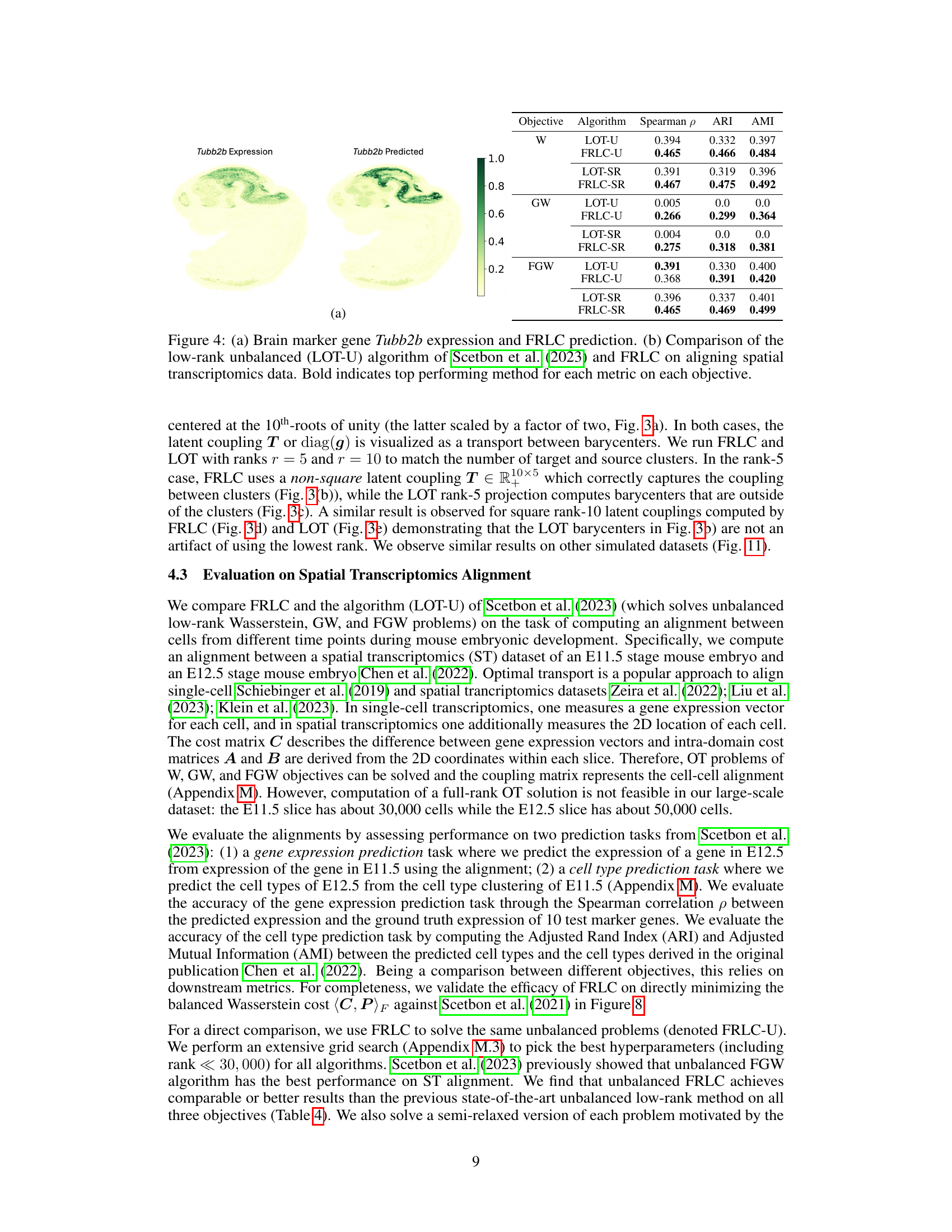
This figure shows the results of comparing FRLC and LOT-U on aligning spatial transcriptomics data. Panel (a) displays the expression of the Tubb2b gene (a brain marker) and its prediction using FRLC. Panel (b) provides a table comparing the performance of LOT-U and FRLC (both unbalanced and semi-relaxed versions) across different optimal transport objectives (Wasserstein, Gromov-Wasserstein, Fused Gromov-Wasserstein) using Spearman correlation, Adjusted Rand Index (ARI), and Adjusted Mutual Information (AMI) metrics. FRLC demonstrates better performance across most metrics and objectives.

This figure shows the convergence rate of the FRLC algorithm on the synthetic dataset of two moons and eight Gaussians. The transport cost is plotted against the number of iterations for both rank-2 and full-rank initializations. The figure shows that the algorithm converges smoothly to a minimum cost, regardless of initialization, demonstrating its robustness and efficiency.

This figure shows the results of comparing FRLC and LOT on three datasets. The first subfigure (a) shows a simulated dataset with two moons and eight Gaussian distributions. The second subfigure (b) shows the transport cost achieved by both algorithms on the dataset in (a) for different ranks and initializations, with FRLC showing better performance. The third subfigure (c) displays results for a 10-dimensional mixture of Gaussians.

This figure shows the results of comparing FRLC and LOT on three different datasets. The first subfigure (a) shows a simulated dataset with two moons and eight Gaussian clusters. Subfigures (b) and (c) present the transport cost results on the dataset from (a) and a 10-dimensional Gaussian mixture, respectively, for varying ranks and different initialization methods. The results indicate that FRLC achieves a lower transport cost than LOT across different ranks and initialization strategies.

This figure shows results comparing FRLC and LOT for solving the balanced Wasserstein problem on a simulated dataset (two moons and eight Gaussians) and a 10D mixture of Gaussians. Subfigure (a) visualizes the simulated dataset. Subfigure (b) presents a plot showing the transport cost achieved by both methods across a range of ranks and different initialization strategies. FRLC demonstrates superior performance across all ranks, achieving lower transport costs than LOT, especially with the full-rank random initialization. Subfigure (c) displays analogous results for a 10D mixture of Gaussians dataset, further supporting FRLC’s superior performance.

This figure visualizes the cell type classification of mouse embryos at two different developmental stages (E11.5 and E12.5). Each cell is color-coded according to its assigned cell type using the annotations provided by Chen et al. (2022) in their spatial transcriptomics study. This visualization aids in understanding the spatial organization and distribution of different cell types during the mouse embryonic development.

This figure compares the ground truth cell type classification of the E12.5 mouse embryo with the cell type classification predicted by the FRLC algorithm. The images show a visual representation of the cell types in two different spatial transcriptomics datasets. The left image is the ground truth, and the right is the prediction made by the FRLC algorithm.
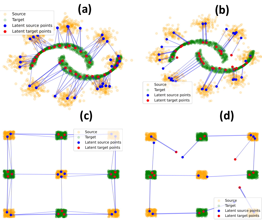
This figure shows the LC-projection barycenters for both FRLC and LOT (Scetbon et al., 2021) on four different datasets. It demonstrates that FRLC latent coupling T captures the coupling between clusters more accurately than LOT diagonal coupling diag(g), especially in the case with non-square latent coupling (T ∈ R10×5).

This figure visualizes the latent coupling learned by FRLC and compares it with the diagonal coupling from Scetbon et al. (2021). It shows the LC-projection barycenters for both methods on four different datasets: two moons and eight Gaussians, and a checkerboard dataset. The results demonstrate that FRLC’s latent coupling better captures the cluster structure of the data compared to the diagonal coupling. Additionally, it’s shown that FRLC’s latent coupling can be diagonalized to recover the factored coupling of Forrow et al. (2019).
More on tables

This table compares several low-rank optimal transport methods, namely those by Forrow et al. (2019), Lin et al. (2021), Scetbon et al. (2021), and the proposed FRLC method. For each method, it lists the type of factorization used for the transport plan (factored coupling or latent coupling), the cost function minimized (Wasserstein barycenter or primal OT cost), the variables optimized, the type of algorithm used, and the subroutine used for computing the coupling.
This table compares several low-rank optimal transport methods: Forrow et al. (2019), Latent OT (Lin et al. 2021), LOT (Scetbon et al. 2021), and FRLC (this work). It contrasts their factorization approach (factored coupling vs. latent coupling), the cost function minimized, the variables used in the optimization, the main algorithm used, and the subroutine used to handle couplings.

This table compares four different low-rank optimal transport methods: Forrow et al. (2019), Latent OT (Lin et al., 2021), LOT (Scetbon et al., 2021), and FRLC (this work). For each method, it lists the type of factorization used (factored coupling or latent coupling), the cost function minimized (Wasserstein, k-Wasserstein barycenter, or primal OT cost), the variables optimized (anchors and sub-couplings, or sub-couplings and inner marginal), the main algorithm used (Lloyd-type, Dykstra’s, mirror descent, or coordinate mirror descent), and the subroutine for coupling. The table highlights the differences in the approach to optimizing low-rank optimal transport plans among the various methods.
This table compares four different low-rank optimal transport methods: Forrow et al. (2019), Latent OT (Lin et al., 2021), LOT (Scetbon et al., 2021), and FRLC (this work). For each method, it lists the type of factorization used for the coupling matrix, the cost function minimized, the variables optimized, and the optimization algorithm used. The table highlights the differences in how each method approaches the problem of low-rank optimal transport, including the choice of factorization and optimization technique.

This table compares the runtime and performance of FRLC and LOT on three synthetic datasets (two moons and 8 Gaussians, 2D Gaussian mixture, and 10D Gaussian mixture) containing 1000 samples each. It reports the CPU time in seconds, the cost value ((C, P)F), and the marginal tightness (||P1n - a||2 and ||PT1m - b||2) for each method and dataset. The FRLC parameters used are specified in the caption.

This table compares the performance of three different graph partitioning methods: GWL, SpecGWL, and the proposed FRLC (semi-relaxed) method. The performance metric used is the Adjusted Mutual Information (AMI). The table shows the AMI scores achieved by each method on four different real-world graph datasets, each tested with four different configurations (symmetric/asymmetric and raw/noisy). The best performing method for each dataset and configuration is highlighted in bold, indicating that the proposed FRLC method often outperforms existing methods in this task.

This table compares the runtime and optimal transport cost of FRLC and LOT on three Stereo-Seq mouse embryo datasets (E9.5-10.5, E10.5-11.5, E11.5-12.5). The results show that FRLC achieves lower optimal transport costs in less time than LOT for all three datasets.
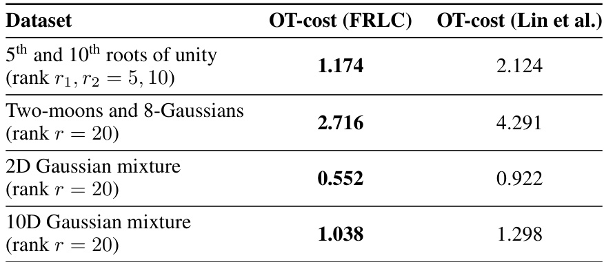
This table compares the primal optimal transport cost achieved by FRLC against the results reported by Lin et al. (2021) on four different synthetic datasets. The datasets include mixtures of Gaussians and two moons. The results show that FRLC consistently achieves a lower optimal transport cost than Lin et al.’s method, highlighting the effectiveness of FRLC in minimizing the primal OT cost.

This table shows the hyperparameters used in a hyperparameter search for validation. It lists the ranges explored for rank (for both FRLC and LOT algorithms), the penalty parameter τ (for FRLC), and the penalty parameters τ and ε (for the LOT-U algorithm). Note that the ranges of τ and τ’ are designed to be similar.
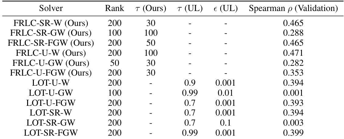
This table shows the best hyperparameter settings found during the validation phase for different low-rank optimal transport algorithms (FRLC and LOT). For each algorithm and objective function (Wasserstein, Gromov-Wasserstein, Fused Gromov-Wasserstein), the table lists the rank of the low-rank approximation used, the hyperparameters (tau, tau prime, epsilon), and the resulting Spearman correlation (a measure of performance) on the validation set. The table is useful for understanding the optimal hyperparameters in different settings, as well as for comparing FRLC and LOT performance.
Full paper#
