TL;DR#
Many real-world tasks are complex and require breaking them down into smaller, manageable subtasks. Current methods often struggle to identify these subtasks effectively, hindering the development of robust and data-efficient AI systems. Existing approaches often rely on heuristics or graphical models that don’t accurately reflect the data generation process, leading to suboptimal results.
This paper proposes a novel method, Sequential Non-negative Matrix Factorization (seq-NMF), which addresses these issues by explicitly modeling the selection mechanism underlying subtask generation. By identifying selection variables that serve as subgoals, seq-NMF efficiently learns meaningful subtasks and demonstrates significant improvements in generalization to new tasks compared to state-of-the-art methods. The experiments demonstrate that the approach effectively enhances generalization in multi-task imitation learning scenarios.
Key Takeaways#
Why does it matter?#
This paper is crucial for researchers in reinforcement learning and artificial intelligence as it provides a novel approach to subtask discovery, a critical challenge in tackling complex tasks. The proposed method, based on identifying selection variables, offers improved data efficiency and generalization capabilities. This work opens new avenues for research in hierarchical reinforcement learning, particularly in developing more robust and adaptable AI systems.
Visual Insights#

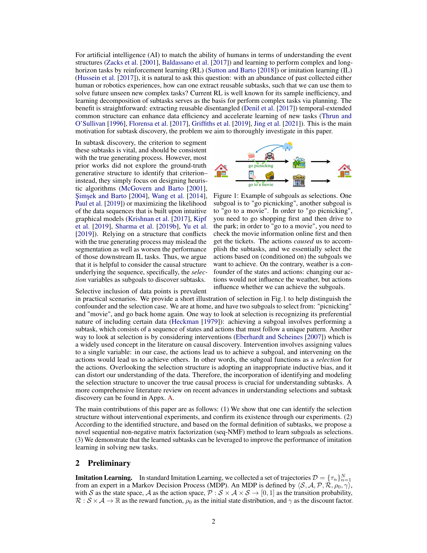
🔼 This figure illustrates the concept of subgoals as selections in contrast to confounders. Two example subgoals are ‘go picnicking’ and ‘go to a movie’. The actions taken to achieve each subgoal are different (shopping and driving vs. checking movie information online and getting tickets). Weather is presented as a confounder, as it influences the states and actions, but is not influenced by them.
read the caption
Figure 1: Example of subgoals as selections. One subgoal is to 'go picnicking', another subgoal is to 'go to a movie'. In order to 'go picnicking', you need to go shopping first and then drive to the park; in order to 'go to a movie', you need to check the movie information online first and then get the tickets. The actions caused us to accomplish the subtasks, and we essentially select the actions based on (conditioned on) the subgoals we want to achieve. On the contrary, weather is a confounder of the states and actions: changing our actions would not influence the weather, but actions influence whether we can achieve the subgoals.

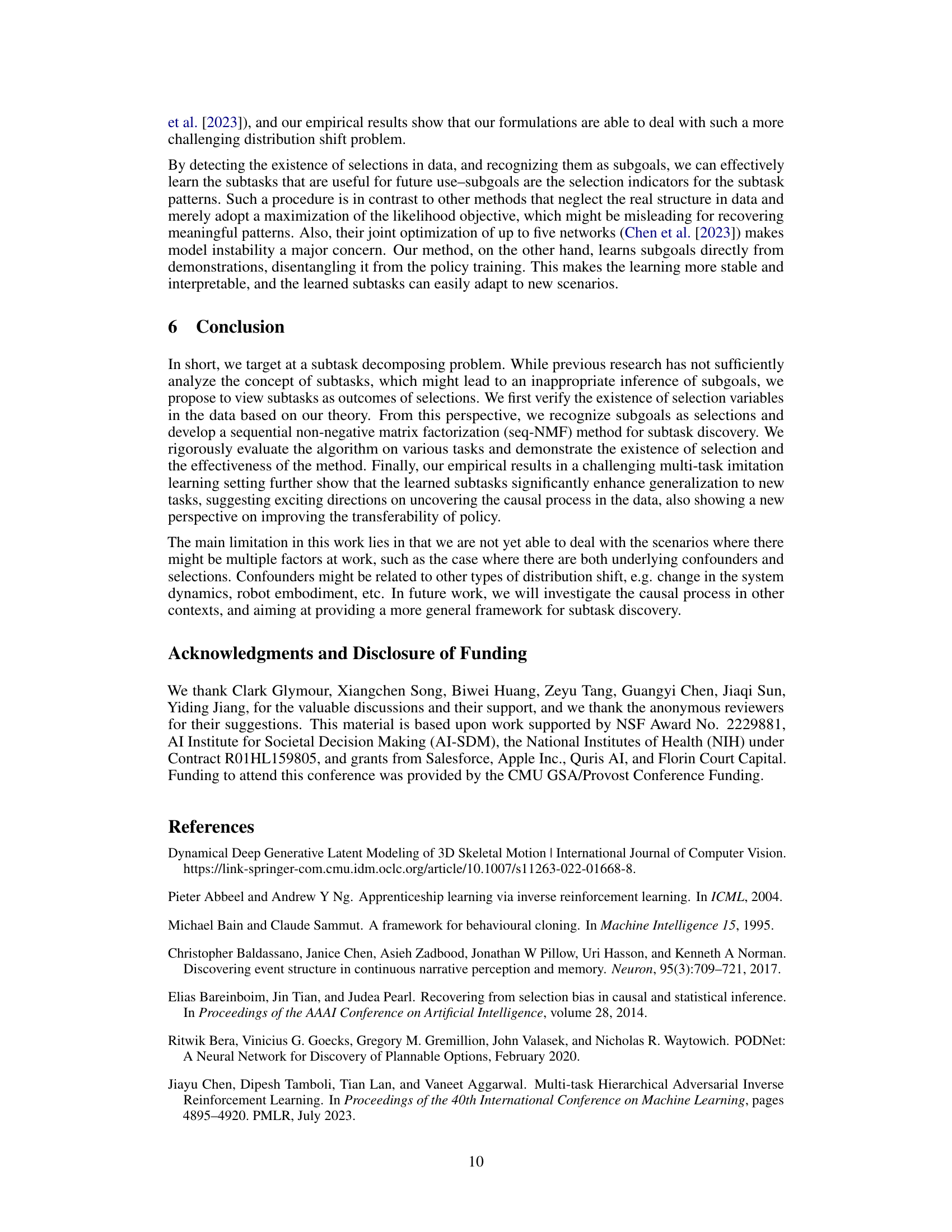
🔼 This table presents the results of three conditional independence (CI) tests performed on the Driving dataset to verify whether subgoals can be identified as selections. The tests assess the conditional independence of variables based on the presence or absence of subgoals. The p-values indicate the significance of the relationships, with lower values suggesting stronger dependence and supporting the hypothesis that subgoals function as selections.
read the caption
Table 1: P-values for CI tests in Driving.
In-depth insights#
Subgoal Selection#
The concept of subgoal selection is central to the paper’s approach to unsupervised subtask discovery. It posits that subtasks aren’t merely intermediate steps but rather outcomes of a selection mechanism driven by subgoals. This contrasts with existing methods which often overlook this underlying structure, focusing instead on heuristics or likelihood maximization. The paper argues that identifying and modeling these selection variables (subgoals) is key to uncovering the true data generation process and extracting meaningful subtasks. This framework allows for a more accurate representation of subtasks, leading to improved data efficiency and better generalization to new tasks. The authors propose a novel method to identify and utilize these subgoals, demonstrating their effectiveness in enhancing the performance of imitation learning in challenging scenarios.
Seq-NMF Method#
The Seq-NMF (Sequential Non-negative Matrix Factorization) method, as described in the research paper, presents a novel approach to unsupervised subtask discovery. It leverages the inherent structure of sequential data, specifically the presence of selection variables acting as subgoals, to decompose long-horizon tasks into meaningful subtasks. The method’s core innovation lies in its ability to identify these selection variables without requiring interventional experiments, which is a significant advantage over existing methods. By modeling subgoals as selections, Seq-NMF directly addresses the true data generation process, resulting in more accurate and robust subtask identification. The method employs a sequential variant of NMF, effectively capturing temporally extended patterns within the data and linking them to the identified subgoals. The resulting subtasks enhance the generalization capabilities of imitation learning models, as demonstrated through empirical evaluations. This approach provides a theoretically grounded and practically effective solution for learning reusable and transferable subtasks, thus overcoming limitations of previous heuristic methods. Furthermore, the incorporation of regularization terms within the Seq-NMF optimization ensures that the identified subtasks are both interpretable and non-redundant, which is critical for effective utilization in downstream tasks. The method also demonstrates a robust solution for subtask ambiguity. Overall, the proposed Seq-NMF method offers a significant improvement in subtask discovery within imitation learning and provides a new perspective on hierarchical planning for complex tasks.
Kitchen Transfer#
The heading ‘Kitchen Transfer’ likely refers to a section detailing the experimental results of applying the proposed method (likely a novel subtask discovery and transfer learning approach) to the challenging Kitchen environment benchmark. This benchmark’s complexity stems from its long-horizon tasks requiring sequential manipulation of multiple objects. The results in this section would demonstrate the ability of the learned subtasks to generalize to new, unseen tasks within the Kitchen environment. Success would show that the subtasks, learned from a limited set of demonstrations, are transferable and reusable in novel task contexts. Conversely, failure to transfer would highlight limitations of the learned representations or the method’s generalizability. The evaluation likely includes comparison to existing hierarchical reinforcement learning or imitation learning approaches, providing a quantitative assessment of performance. Specific metrics such as cumulative reward, success rate, and learning efficiency are expected to be used for comparison. A detailed analysis of the results would likely be provided, possibly including visualizations or error bars, to show the statistical significance of the findings and their robustness.
Selection Bias#
Selection bias, a critical issue in causal inference and machine learning, significantly impacts the validity of research findings by systematically excluding certain data points. In the context of subtask discovery, selection bias arises when the choice of subtasks is not random but determined by factors correlated with the outcome variable. This leads to skewed representations of the underlying data-generating process, resulting in inaccurate conclusions about the relationships between subtasks and overall task success. Addressing selection bias requires careful consideration of the data collection process. Understanding how subtasks are selected and the potential confounding factors is crucial. Methods like inverse probability weighting (IPW) or matching can help mitigate this bias, but their effectiveness depends on accurate modeling of the selection mechanism. Algorithmic approaches for subtask discovery should explicitly address selection bias. This might involve incorporating techniques from causal inference, such as causal discovery algorithms, or leveraging techniques like propensity score matching to balance the representation of subtasks. Ignoring selection bias can lead to misleading results about the generalization capabilities of learned subtasks and the overall data structure. Therefore, rigorous attention to selection bias is crucial for both theoretical understanding and practical application of unsupervised subtask discovery.
Future Research#
Future research directions stemming from this work on unsupervised subtask discovery could profitably explore several avenues. Extending the framework to handle more complex causal structures involving both confounders and selection variables would enhance the model’s robustness and applicability to a wider array of real-world scenarios. Investigating higher-order subgoal hierarchies and developing methods to learn these structures would improve the model’s ability to decompose complex tasks into manageable subtasks. Another important area is improving the generalization capability of learned subtasks to novel tasks, perhaps by incorporating methods for transfer learning and domain adaptation. Further research should focus on evaluating the approach on more diverse and challenging tasks within different domains (robotics, game playing, etc.) to better understand its strengths and limitations. Finally, exploring alternative methods for subtask representation and learning, such as deep generative models, might yield further insights and improved performance. A detailed analysis of the relationship between subgoal selection and reward learning could also lead to significant advancements in the field of hierarchical reinforcement learning.
More visual insights#
More on figures

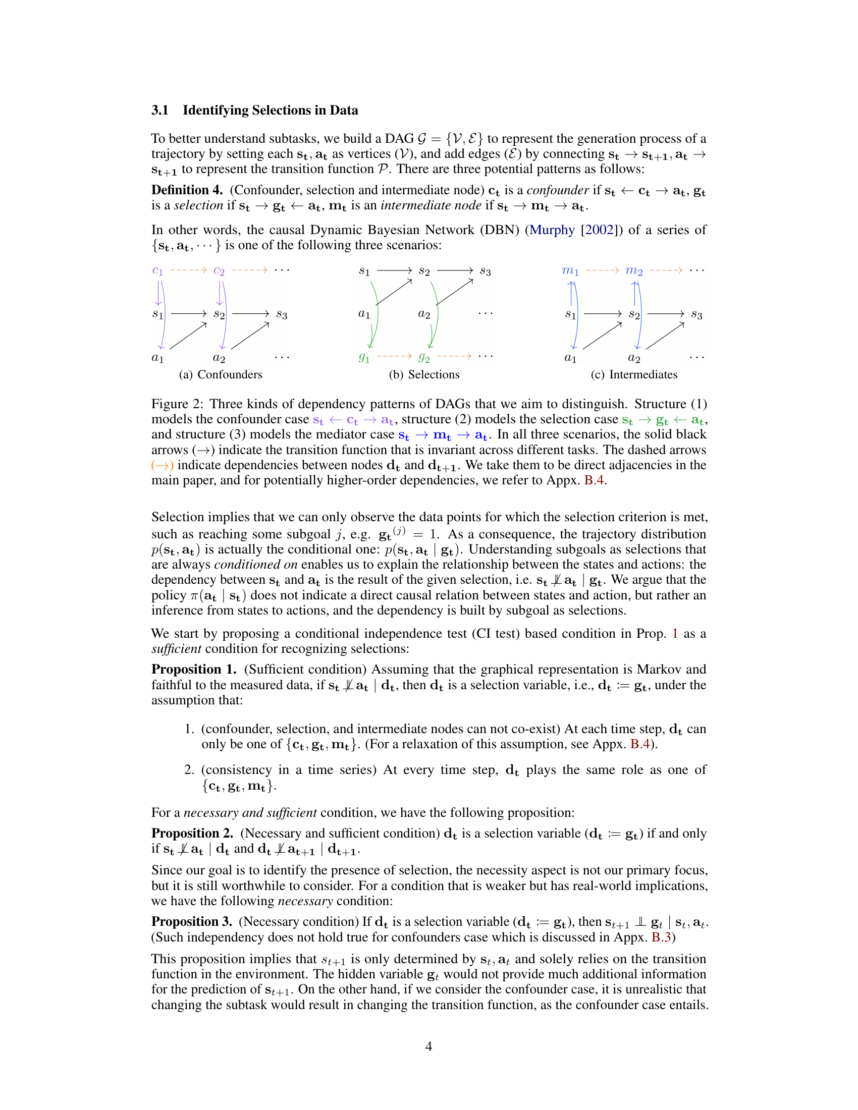
🔼 This figure illustrates three different causal relationships between states (s), actions (a), and a third variable (c, g, or m), representing confounders, selections, and intermediates, respectively. The solid arrows represent the transition function, consistent across tasks. Dashed arrows show relationships between time steps. The figure is crucial for understanding how to distinguish between a selection variable (representing subgoals) and other variables to identify subtasks accurately.
read the caption
Figure 2: Three kinds of dependency patterns of DAGs that we aim to distinguish. Structure (1) models the confounder case St← Ctat, structure (2) models the selection case st → gt ← at, and structure (3) models the mediator case stmt → at. In all three scenarios, the solid black arrows (→) indicate the transition function that is invariant across different tasks. The dashed arrows (→) indicate dependencies between nodes dt and dt+1. We take them to be direct adjacencies in the main paper, and for potentially higher-order dependencies, we refer to Appx. B.4.
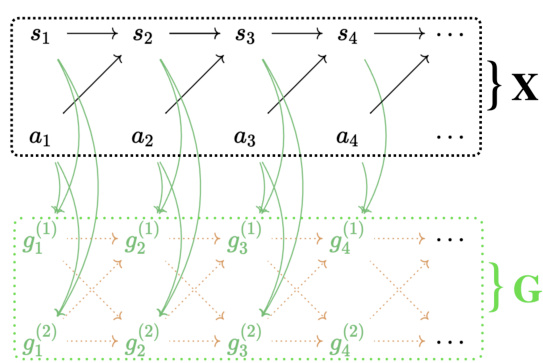
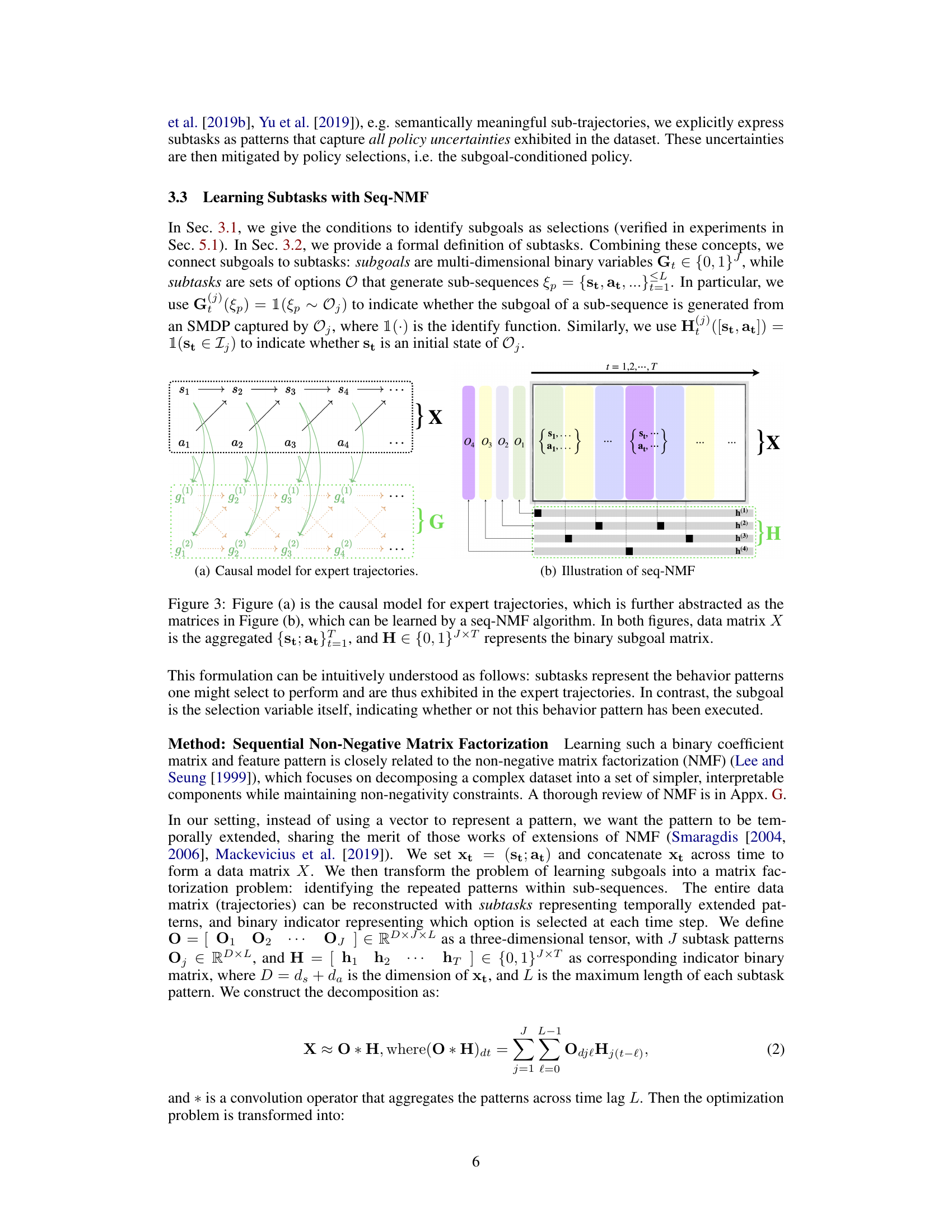
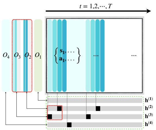
🔼 This figure illustrates the causal model for expert trajectories and its matrix factorization representation using seq-NMF. (a) shows a causal graph where states (s), actions (a), and subgoals (g) influence each other. (b) presents the seq-NMF abstraction of this model, representing the data as a matrix X and decomposing it into a feature pattern matrix O (subtasks) and a binary coefficient matrix H (subgoal selections). Seq-NMF learns both the subtask patterns and their selection indicators to represent the expert demonstrations.
read the caption
Figure 3: Figure (a) is the causal model for expert trajectories, which is further abstracted as the matrices in Figure (b), which can be learned by a seq-NMF algorithm. In both figures, data matrix X is the aggregated {st; at}t=1, and H ∈ {0,1}J×T represents the binary subgoal matrix.
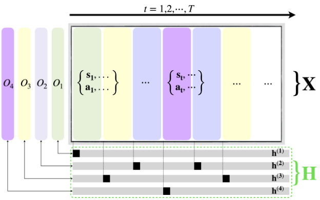
🔼 This figure illustrates the causal model for expert trajectories and its matrix factorization using seq-NMF. Figure (a) shows a causal graph representing the generation of expert trajectories, where states (st), actions (at), and subgoals (gt) are depicted as nodes and their relationships as directed edges. Figure (b) provides a simplified representation using matrices: X represents the aggregated state-action pairs, and H is a binary matrix indicating the presence or absence of subgoals for each subtask. The seq-NMF algorithm learns these matrices to identify subtasks from the data.
read the caption
Figure 3: Figure (a) is the causal model for expert trajectories, which is further abstracted as the matrices in Figure (b), which can be learned by a seq-NMF algorithm. In both figures, data matrix X is the aggregated {st; at}t=1, and H ∈ {0,1}J×T represents the binary subgoal matrix.

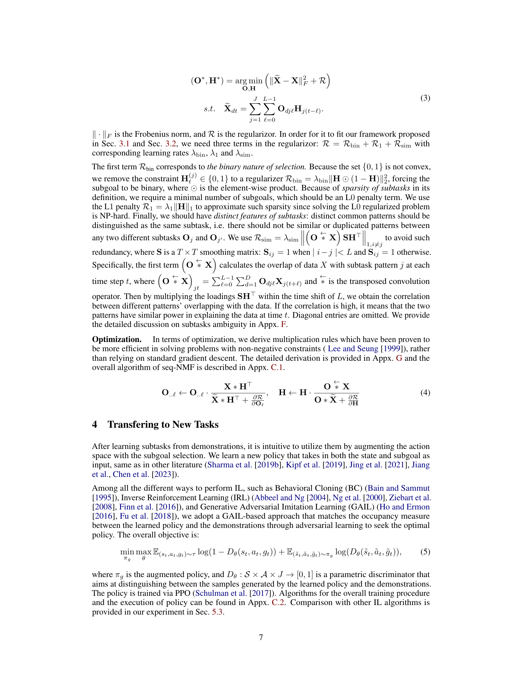
🔼 This figure shows two different patterns used in the synthetic Color dataset. Color-3 has three colors (red, yellow, blue) each repeated three times, and Color-10 has two patterns: (3 red, 3 yellow, 4 blue) and (3 blue, 3 yellow, 4 red), each with 10 steps. These patterns are used to evaluate the causal inference methods. The figure illustrates the repeating nature of the color patterns and serves to visually represent the data structure used in the experiment.
read the caption
Figure 4: Patterns in Color-3 and -10.

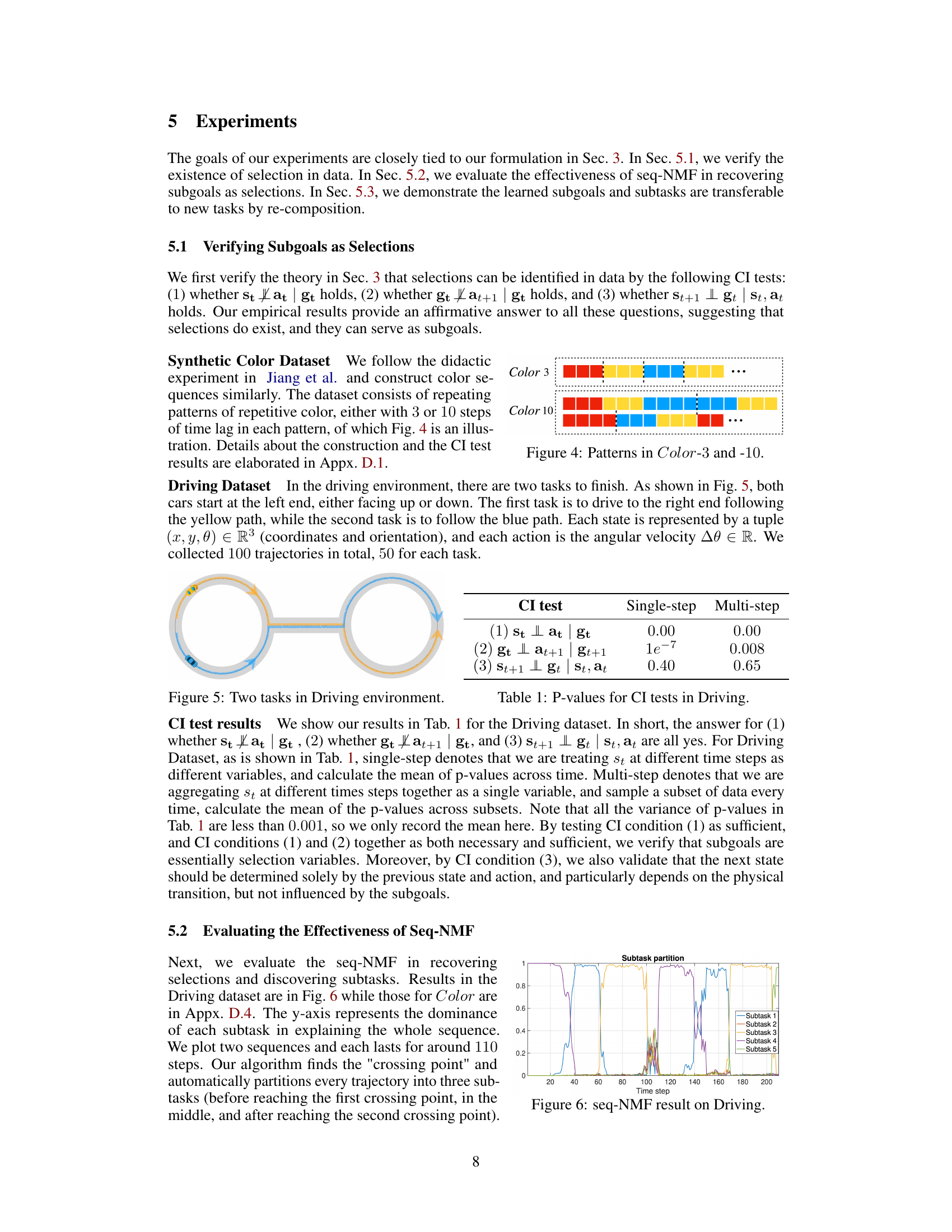
🔼 This figure shows two different driving tasks in a simulated environment. Both tasks start with two cars positioned at the left end of a track, but one car faces upwards while the other faces downwards. The first task requires the car to follow a yellow path to the right end of the track. The second task instructs the car to navigate a blue path to the same destination. Each task involves different routes and navigation challenges, highlighting the complexity and variety in the driving scenarios used for evaluating the proposed method.
read the caption
Figure 5: Two tasks in Driving environment.

🔼 This figure displays the results of applying the sequential non-negative matrix factorization (seq-NMF) method to the Color-10 dataset. The y-axis represents the dominance of each subtask in explaining the whole sequence. The x-axis represents the time steps. The graph shows five different colored lines representing the five subtasks identified by the algorithm. The dominance of each subtask varies over time, indicating how much each subtask contributes to the overall sequence at different points. The plot visually demonstrates the algorithm’s ability to partition the trajectory into meaningful subtasks.
read the caption
Figure 14: seq-NMF result on Color-10. The dominance of each subtask in explaining 10 sequences.

🔼 This figure shows the Kitchen environment used in the experiments. It is a simulated kitchen setting with a robot arm, microwave, stove, sink, and cabinets. The robot arm is the agent that performs the tasks in the environment. The environment is used to test the ability of the learned subtasks to generalize to new tasks.
read the caption
Figure 7: Kitchen environment

🔼 The figure shows the results of four different imitation learning methods on two new tasks in the Kitchen environment. The x-axis represents the total number of training steps, while the y-axis represents the accumulated return. The four methods are Ours, DI-GAIL, H-AIRL, and Option-GAIL. Each method is represented by a line and shaded area, which represents the mean and standard deviation across five independent runs. The figure demonstrates that the proposed method outperforms the baselines in terms of both efficiency and performance on solving the new tasks. In particular, the proposed method can effectively transfer the knowledge learned from the demonstrations to the new tasks and quickly adapts to the tasks with different compositions of subtasks.
read the caption
Figure 8: Results for solving new tasks in the Kitchen environment w.r.t. training steps.
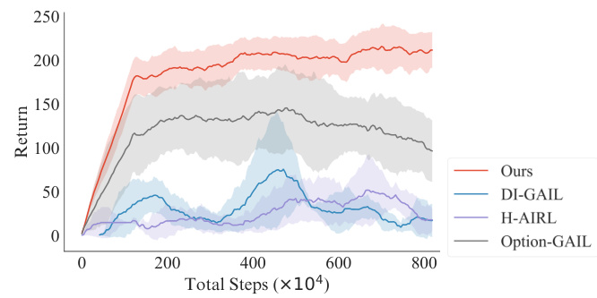
🔼 This figure shows the results of applying different imitation learning methods to solve new tasks in the Kitchen environment. The x-axis represents the total number of training steps, and the y-axis represents the episodic accumulated reward. The graph displays the performance of four methods: ‘Ours’, ‘DI-GAIL’, ‘H-AIRL’, and ‘Option-GAIL’. The shaded area around each line represents the standard deviation across multiple training runs. The results indicate how quickly each method adapts to new tasks with different compositions of subtasks.
read the caption
Figure 8: Results for solving new tasks in the Kitchen environment w.r.t. training steps.

🔼 Figure 3 shows two representations of the causal model for expert trajectories. (a) is a graphical representation showing the causal relationships between states (st), actions (at), and subgoals (gt). Dashed arrows indicate the temporal dependence between timesteps. (b) provides a more abstract, matrix representation of the same causal model. Here, data matrix X represents the combined states and actions across time, while matrix H (a binary matrix) indicates whether a particular subgoal is active at each time step. This matrix factorization simplifies the learning process.
read the caption
Figure 3: Figure (a) is the causal model for expert trajectories, which is further abstracted as the matrices in Figure (b), which can be learned by a seq-NMF algorithm. In both figures, data matrix X is the aggregated {st; at}t=1, and H ∈ {0,1}J×T represents the binary subgoal matrix.
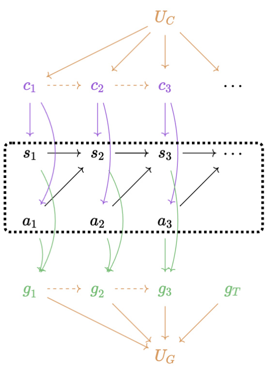
🔼 This figure presents a graphical model illustrating the data generation process. It relaxes the assumptions made in Figure 2 by allowing for the co-existence of confounders (c), selections (g), and mediators (m) at each time step. Additionally, it incorporates higher-order structures, denoted by Uc (higher-order confounders) and Ug (higher-order selections). These higher-order structures influence the relationships between the variables at each time step, creating more complex dependencies. The figure shows how these higher-order variables affect the relationships between states (s), actions (a), and subgoals (g).
read the caption
Figure 11: Graphical model with relaxed assumptions. (1) We allow the co-existance of gt and ct (similarly for gt and mt). (2) We also assume there are potential higher-order underlying confounders Uc in the data that create the dependencies between ct and ct+1, and underlying selections Us in the data that create the dependencies between gt and ct+1.
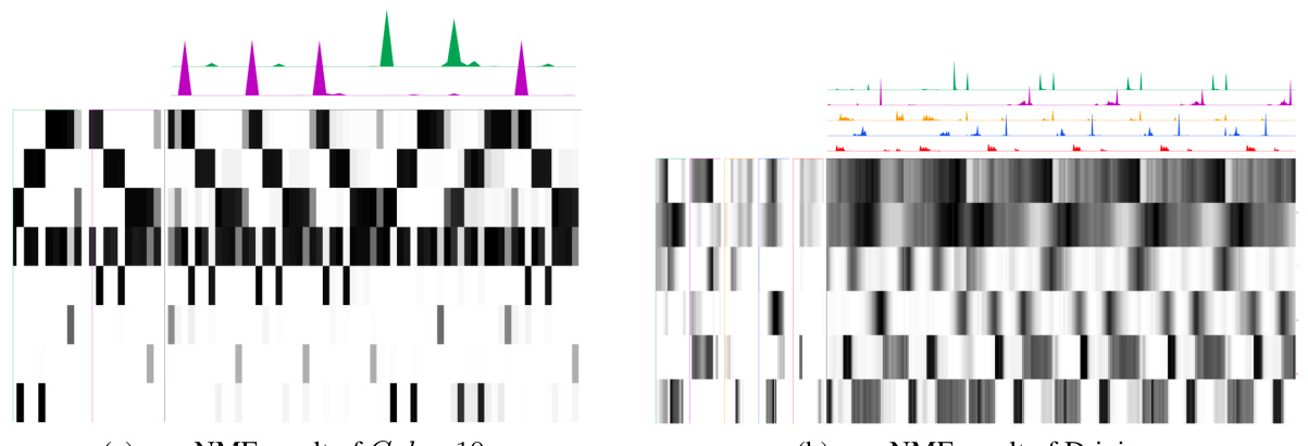
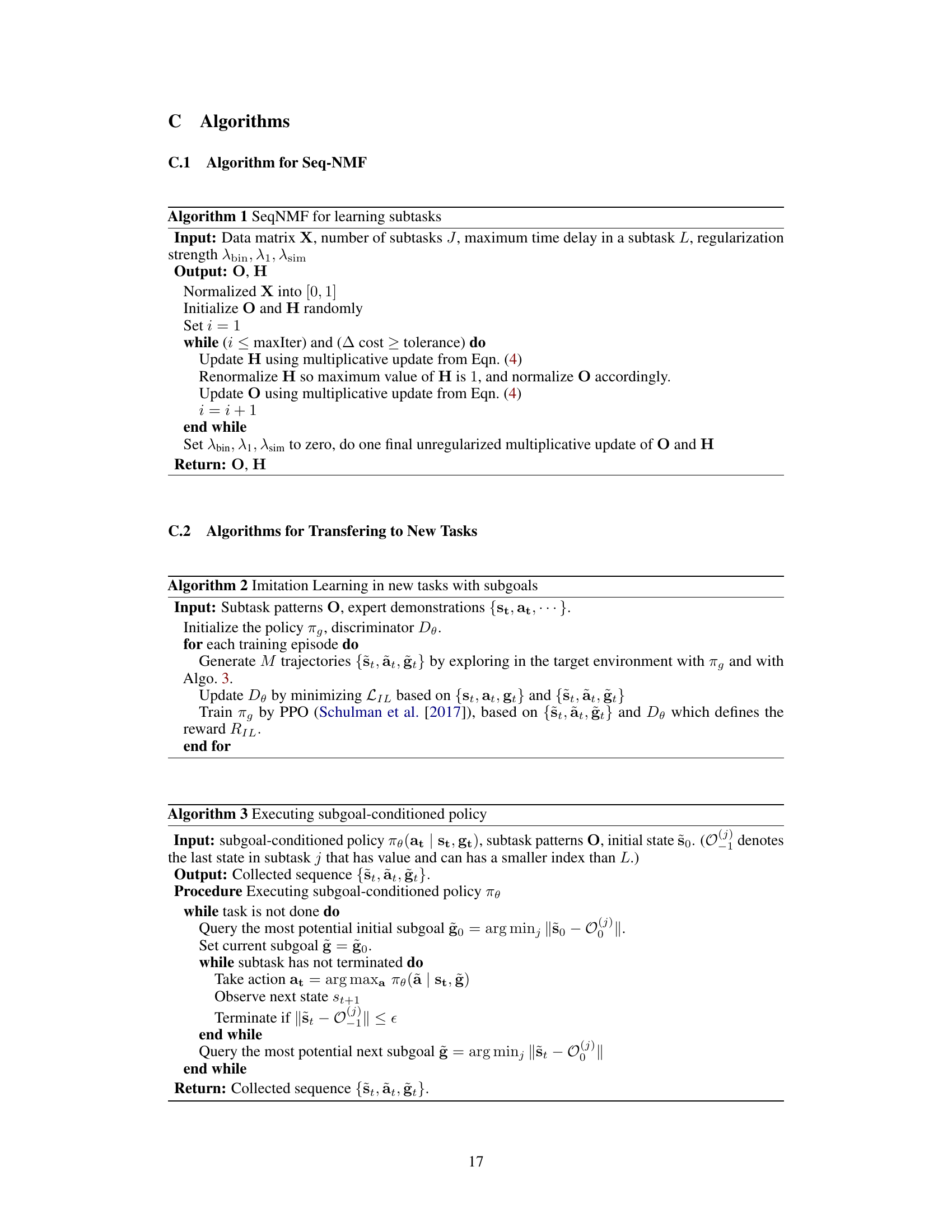
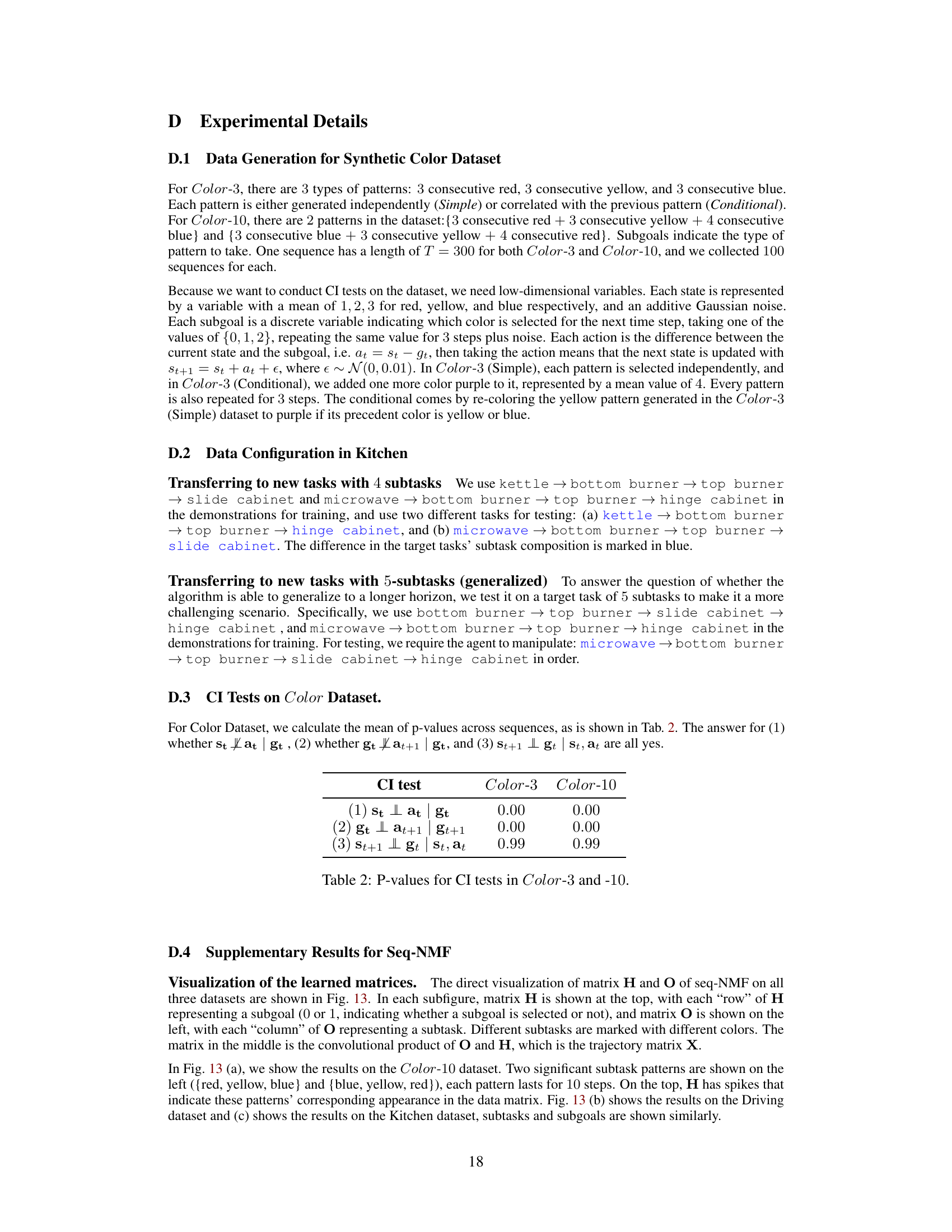
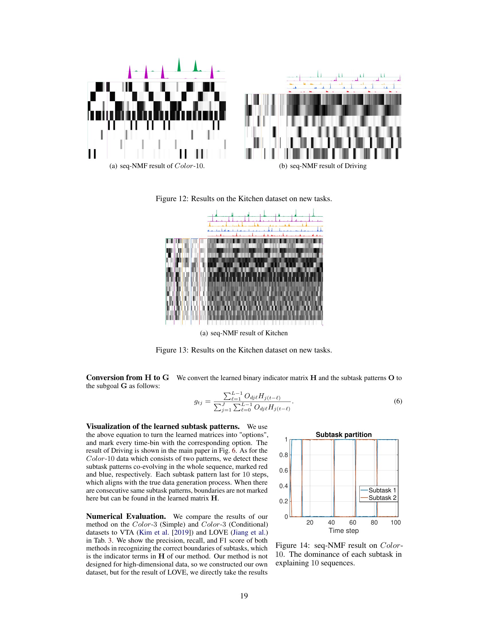
🔼 This figure presents the results of applying seq-NMF on the Kitchen dataset for new tasks. It visualizes the learned binary indicator matrix H (subgoals) and the subtask patterns O. The matrix in the middle is the convolutional product of O and H, representing the trajectory matrix X. Different subtask patterns are shown using different colors. For each subfigure, the dominance of each subtask in explaining the whole sequence is shown. The figure helps to demonstrate the effectiveness of seq-NMF in recovering selections and discovering subtasks in a complex real-world scenario.
read the caption
Figure 13: Results on the Kitchen dataset on new tasks.
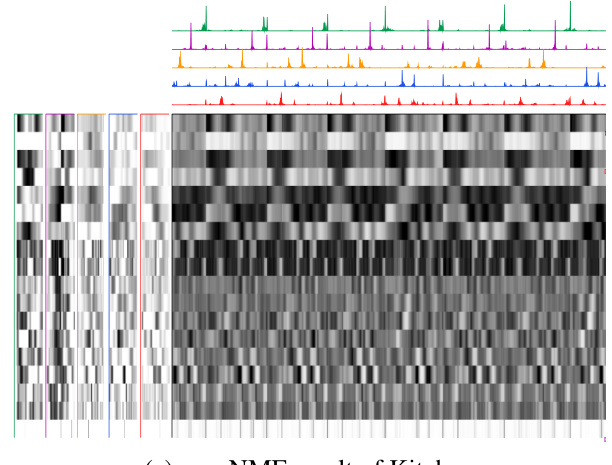
🔼 This figure shows the results of applying seq-NMF to the Kitchen dataset. The top section displays the learned binary indicator matrix H, representing the selection of subtasks. Each row corresponds to a different subgoal, and a value of 1 indicates the subgoal was selected at that timestep. The bottom section shows the learned subtask patterns O, represented as a matrix. Each column corresponds to a distinct subtask pattern. The middle section shows the reconstruction of the data matrix X using the learned subtasks. This visualization demonstrates how the algorithm identifies and separates different subtask patterns within the kitchen dataset.
read the caption
Figure 13: Results on the Kitchen dataset on new tasks.
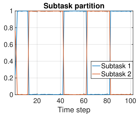
🔼 This figure displays the results of applying the sequential non-negative matrix factorization (seq-NMF) method to the Color-10 dataset. The y-axis represents the dominance of each subtask in explaining the overall sequence, indicating how much each subtask contributes to the different parts of the sequence. The x-axis represents the time steps. The plot shows the dominance of two subtasks over the sequence, suggesting the identification of two main patterns within the dataset.
read the caption
Figure 14: seq-NMF result on Color-10. The dominance of each subtask in explaining 10 sequences.
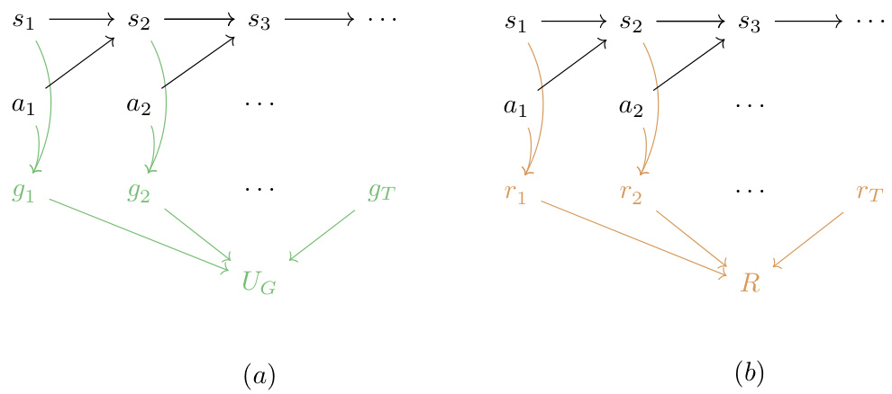
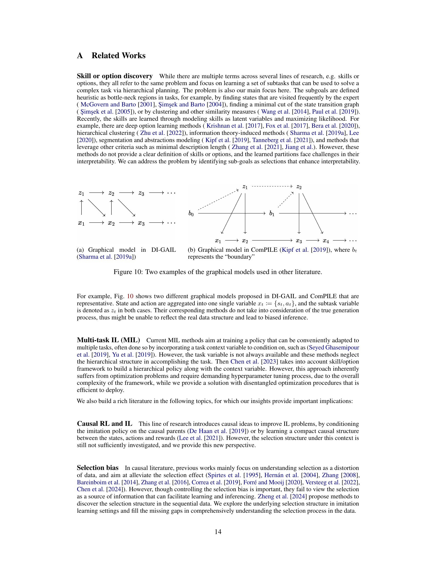
🔼 This figure showcases two graphical models from existing literature (DI-GAIL and ComPILE). Both models represent attempts to discover subtasks or options, but they differ in their approach to modeling the data and the subtasks. The key difference lies in whether or not they consider the true data generating process, which can lead to biased inference if not considered. The figure highlights the importance of accurately modeling the data generation process for effective subtask discovery.
read the caption
Figure 10: Two examples of the graphical models used in other literature.

🔼 Figure 3 presents a graphical model representing expert trajectories (a) which is further abstracted into matrices (b) used in the seq-NMF algorithm. (a) shows the causal relationships between states (s), actions (a), and subgoals (g) in an expert trajectory. These relationships are then represented in matrix form in (b). Matrix X represents the aggregated state-action pairs. The matrix H (binary) indicates the presence or absence of a subgoal for each subtask.
read the caption
Figure 3: Figure (a) is the causal model for expert trajectories, which is further abstracted as the matrices in Figure (b), which can be learned by a seq-NMF algorithm. In both figures, data matrix X is the aggregated {st; at }f=1, and H ∈ {0,1}J×T represents the binary subgoal matrix.
🔼 Figure 3 shows two perspectives of modeling expert trajectories. (a) presents a causal model illustrating the relationships between states (st), actions (at), and subgoals (gt). (b) provides an abstract representation of this model using matrices for seq-NMF processing. Matrix X aggregates states and actions, while matrix H represents binary subgoal selections. The figure highlights how the algorithm uses these matrices to learn behavior patterns and identify subgoals.
read the caption
Figure 3: Figure (a) is the causal model for expert trajectories, which is further abstracted as the matrices in Figure (b), which can be learned by a seq-NMF algorithm. In both figures, data matrix X is the aggregated {st; at}t=1, and H ∈ {0,1}J×T represents the binary subgoal matrix.
More on tables

🔼 This table presents the p-values obtained from three conditional independence (CI) tests performed on the Driving dataset. These tests aim to verify the existence of selection variables (subgoals) in the data. The tests assess the conditional independence between states (st) and actions (at) given the subgoal (gt), the conditional independence between the subgoal (gt) and the next action (at+1) given the next subgoal (gt+1), and the conditional independence between the next state (st+1) and the current subgoal (gt) given the current state (st) and action (at). The results from these tests support the hypothesis that subgoals function as selection variables.
read the caption
Table 1: P-values for CI tests in Driving.

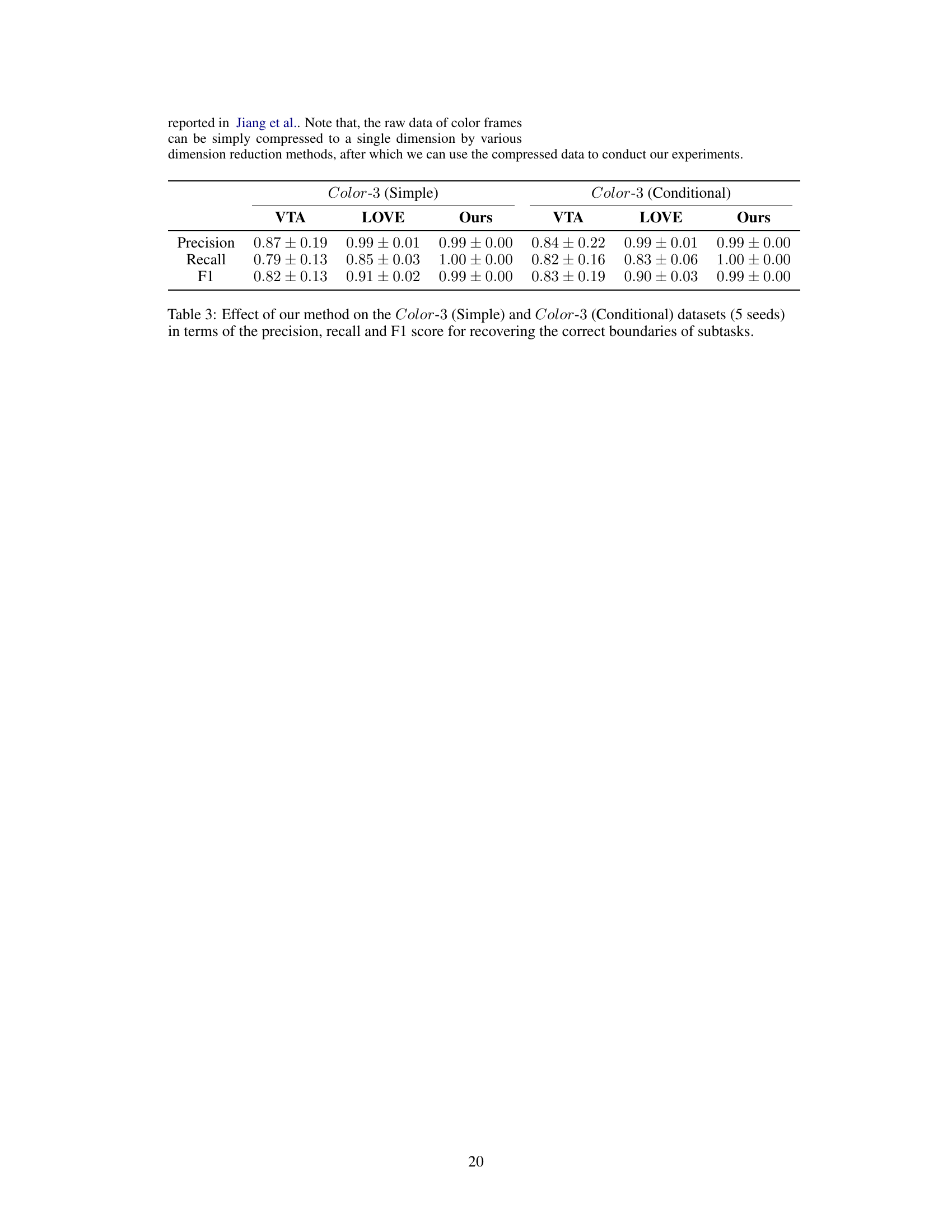
🔼 This table presents the performance comparison of three different methods (VTA, LOVE, and the proposed method) on two datasets (Color-3 Simple and Color-3 Conditional) for subtask boundary detection. The metrics used for comparison are precision, recall, and F1-score. The results show that the proposed method outperforms the other two methods, achieving near-perfect scores.
read the caption
Table 3: Effect of our method on the Color-3 (Simple) and Color-3 (Conditional) datasets (5 seeds) in terms of the precision, recall and F1 score for recovering the correct boundaries of subtasks.
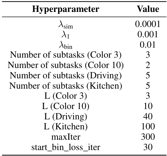
🔼 This table lists the hyperparameters used in the seq-NMF algorithm for learning subtasks. It specifies values for regularization strengths (λsim, λ1, λbin), the number of subtasks for each dataset (Color 3, Color 10, Driving, Kitchen), the maximum time delay in a subtask (L) for each dataset, the maximum number of iterations (maxIter), and the iteration at which to start minimizing the binary loss (start_bin_loss_iter).
read the caption
Table 4: Hyperparameters in seq-NMF

🔼 This table lists the hyperparameters used in the hierarchical imitation learning (IL) part of the experiments. It shows settings for the policy network, the PPO (Proximal Policy Optimization) algorithm, and the discriminator in the Generative Adversarial Imitation Learning (GAIL) framework. Specific hyperparameters include the number of samples per epoch, number of epochs, activation function, hidden layer dimensions, learning rate, and clipping parameters. These settings are crucial for fine-tuning the performance of the imitation learning model in transferring to new tasks.
read the caption
Table 5: Hyperparameters in hierarchical IL
Full paper#
