TL;DR#
Accurate high-resolution precipitation forecasting is computationally expensive using traditional climate models. Statistical downscaling offers a workaround by enhancing low-resolution predictions using statistical methods, but these often fail to capture the accurate distribution of high-resolution data and provide unbiased extreme event estimations. This limitation hinders reliable ensemble averages and can result in inaccurate predictions, especially for events like heavy rain.
The study introduces SpatioTemporal Video Diffusion (STVD), a novel approach that extends video diffusion models for precipitation super-resolution. STVD uses a two-stage process involving a deterministic downscaler followed by a temporally-conditioned diffusion model. This method helps capture noise characteristics and high-frequency precipitation patterns. Experiments on FV3GFS output show that STVD significantly outperforms six state-of-the-art baselines across various metrics, including the continuous ranked probability score (CRPS) and mean squared error (MSE), demonstrating improved accuracy and a superior ability to model precipitation distributions. STVD’s improved accuracy makes it a promising technique for climate modeling, weather forecasting, and disaster preparedness.
Key Takeaways#
Why does it matter?#
This paper is important because it introduces a novel and effective method for improving the accuracy of precipitation predictions, a crucial aspect of climate modeling and forecasting. The approach uses deep learning techniques to upscale low-resolution precipitation data, addressing the computational limitations of traditional high-resolution simulations. This method has the potential to significantly improve our ability to predict and prepare for extreme weather events and inform crucial climate change adaptation strategies.
Visual Insights#

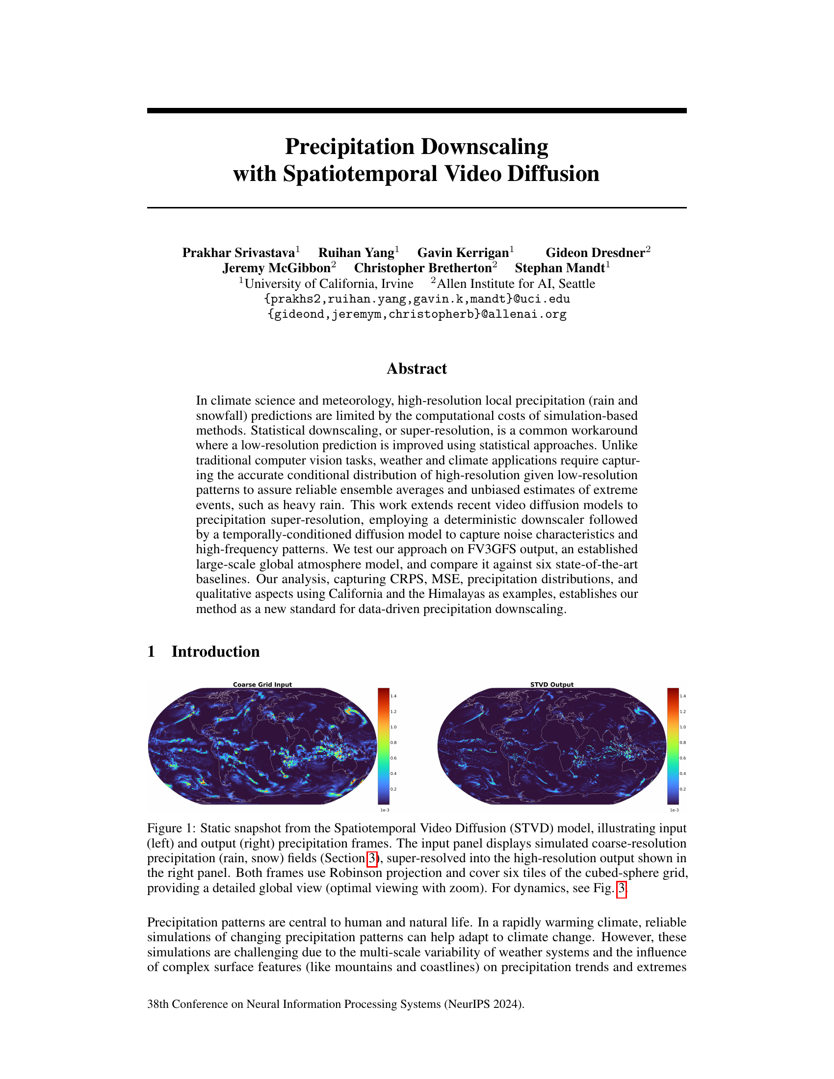
🔼 This figure shows a comparison between the input (low-resolution) and output (high-resolution) precipitation frames generated by the Spatiotemporal Video Diffusion (STVD) model. The left panel displays the coarse-resolution precipitation data as input to the model, while the right panel shows the high-resolution precipitation data generated by STVD as output. Both images use the Robinson projection and cover the entire globe, showcasing the model’s ability to upscale precipitation data from a coarse to a fine resolution.
read the caption
Figure 1: Static snapshot from the Spatiotemporal Video Diffusion (STVD) model, illustrating input (left) and output (right) precipitation frames. The input panel displays simulated coarse-resolution precipitation (rain, snow) fields (Section 3), super-resolved into the high-resolution output shown in the right panel. Both frames use Robinson projection and cover six tiles of the cubed-sphere grid, providing a detailed global view (optimal viewing with zoom). For dynamics, see Fig. 3.

🔼 This table presents a quantitative comparison of the proposed STVD model against six state-of-the-art baselines across multiple metrics. The metrics used are CRPS (Continuous Ranked Probability Score), MSE (Mean Squared Error), EMD (Earth Mover Distance), PE (99.999th percentile error), and SAE (Spatial Autocorrelation Error). The results demonstrate that STVD outperforms all baselines. Additionally, an ablation study shows the impact of removing additional data inputs (STVD-single) or reducing the input sequence length (STVD-3 and STVD-1) on the model’s performance.
read the caption
Table 1: Quantitative comparison between our method and other competitive baselines. EMD represents the Earth-Mover Distance, PE denotes the 99.999th percentile error and SAE is the spatial-autocorrelation error. Overall, our proposed method (STVD) outperforms the baselines across all metrics. In our ablation study, the exclusion of additional side information (STVD-single) or decrement in context length (STVD-3 and STVD-1) appreciably degrades performance.
In-depth insights#
Spatiotemporal Diffusion#
Spatiotemporal diffusion models offer a powerful approach to address challenges in high-resolution prediction tasks by integrating spatial and temporal dependencies. Their ability to handle multi-modal distributions is particularly beneficial in complex systems like weather prediction, where uncertainty and variability are inherent. By combining deterministic downscaling with a diffusion model, spatiotemporal methods can capture both large-scale patterns and high-frequency details, thereby overcoming limitations of traditional statistical approaches. The use of factorized attention mechanisms enhances efficiency and scalability, enabling the processing of extensive spatiotemporal data. However, challenges remain. The need for paired high-resolution/low-resolution training data presents a bottleneck, and ensuring the model’s generalizability to diverse regions and climatic conditions necessitates further investigation. While promising for improved accuracy and uncertainty quantification, careful consideration of computational cost and data requirements is crucial for the practical application of these methods.
Conditional Modeling#
Conditional modeling, in the context of this research paper, is a crucial technique for enhancing the realism and accuracy of precipitation downscaling. It involves learning the conditional probability distribution of high-resolution precipitation data given corresponding low-resolution data. This approach moves beyond deterministic methods that often average out important features. By explicitly modeling the conditional distribution, conditional models can capture the uncertainty inherent in precipitation patterns, leading to more realistic ensemble predictions. This is particularly important for accurately predicting extreme events such as heavy rainfall, which are often underestimated by simpler methods. The use of diffusion models within this conditional framework is a key innovation, as they are capable of modeling complex, high-dimensional distributions effectively. The combination of deterministic downscaling and diffusion-based residual modeling provides a powerful approach that balances the advantages of both, leading to improved accuracy in precipitation forecasts. This multifaceted modeling strategy is superior for diverse climate applications.
Precipitation Downscaling#
Precipitation downscaling tackles the challenge of improving the resolution of climate models’ precipitation predictions. Standard climate models operate at coarser resolutions, insufficient for local-level impact assessments. Downscaling refines these predictions using statistical or dynamical methods, bridging the gap between coarse-resolution predictions and the higher-resolution data needed for applications like flood risk management and agricultural planning. The core challenge lies in accurately capturing the complex statistical relationships between large and small-scale weather patterns. This often involves sophisticated techniques like super-resolution algorithms or the integration of finer-scale data into the models. Success hinges on developing methods that are both accurate and computationally efficient, considering the vast amounts of data involved in climate modeling. The goal is to improve the reliability of local precipitation forecasts, leading to better-informed decision-making in various sectors.
Multi-Scale Variability#
Multi-scale variability in complex systems, such as weather patterns, is a significant challenge for accurate modeling and prediction. It arises from the interaction of processes operating at vastly different spatial and temporal scales, ranging from microphysics of individual cloud droplets to the global circulation of atmospheric winds. Understanding and representing these interactions is crucial for improving the accuracy and reliability of weather forecasts, particularly in predicting extreme weather events like heavy rainfall or droughts. This requires advanced modeling techniques that can resolve both large-scale features and small-scale processes, often relying on nested grids or data assimilation schemes. The high computational cost associated with multi-scale models is a critical barrier. Data-driven methods, such as deep learning, offer a potential pathway to improve efficiency while maintaining accuracy. These methods can capture complex relationships between scales that may be difficult to represent explicitly in traditional models. However, challenges remain in ensuring the generalizability of these methods and accurately representing uncertainty.
Ablation Studies#
Ablation studies systematically remove components of a model to assess their individual contributions. In this context, removing elements like temporal attention or additional input channels (e.g., topography, wind speed) allows for a precise evaluation of their impact on the model’s performance. By comparing the results of the complete model against these ‘ablated’ versions, researchers can determine the importance of each component, isolate sources of error, and identify strengths. Focusing on various aspects such as MSE, CRPS, and extreme precipitation accuracy helps researchers quantify these effects. This detailed analysis provides insights into the model’s architecture, helping to optimize it for better performance, particularly highlighting the robustness and reliability of its elements. The results should clearly demonstrate the significance of the included features in achieving high accuracy and show which features contribute most to the overall performance, which helps in refining model architecture and understanding the model’s capabilities and limitations.
More visual insights#
More on figures
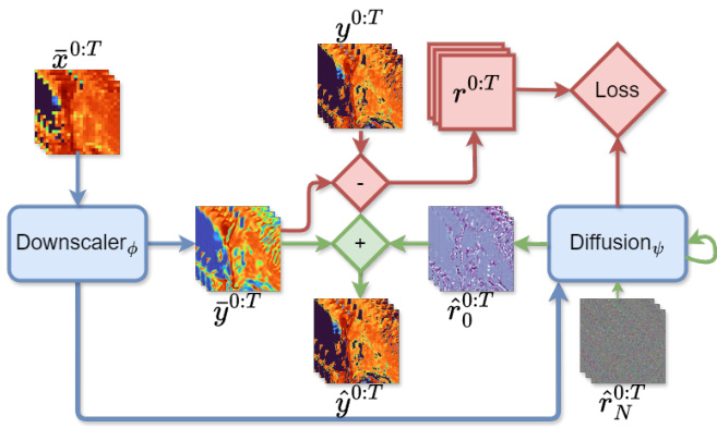
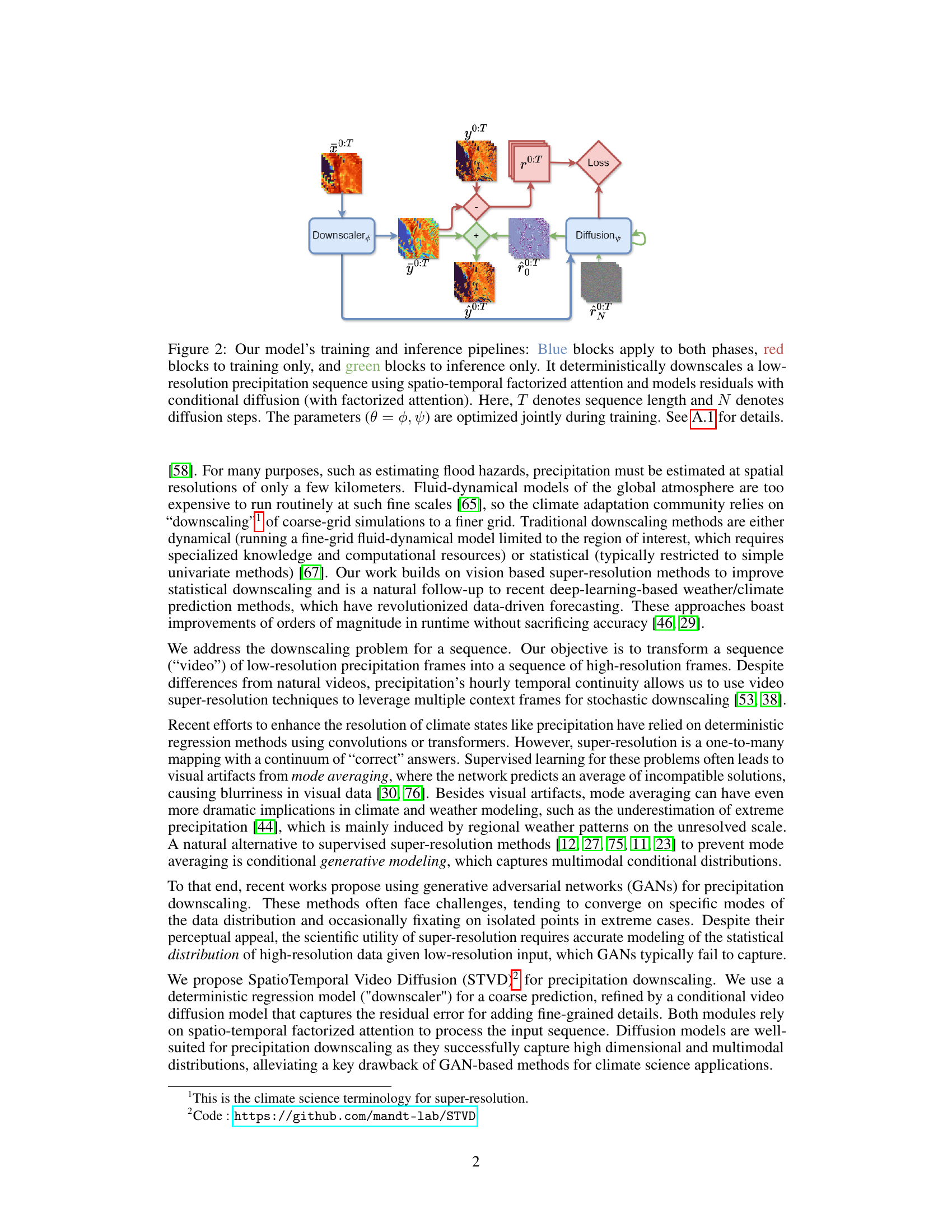
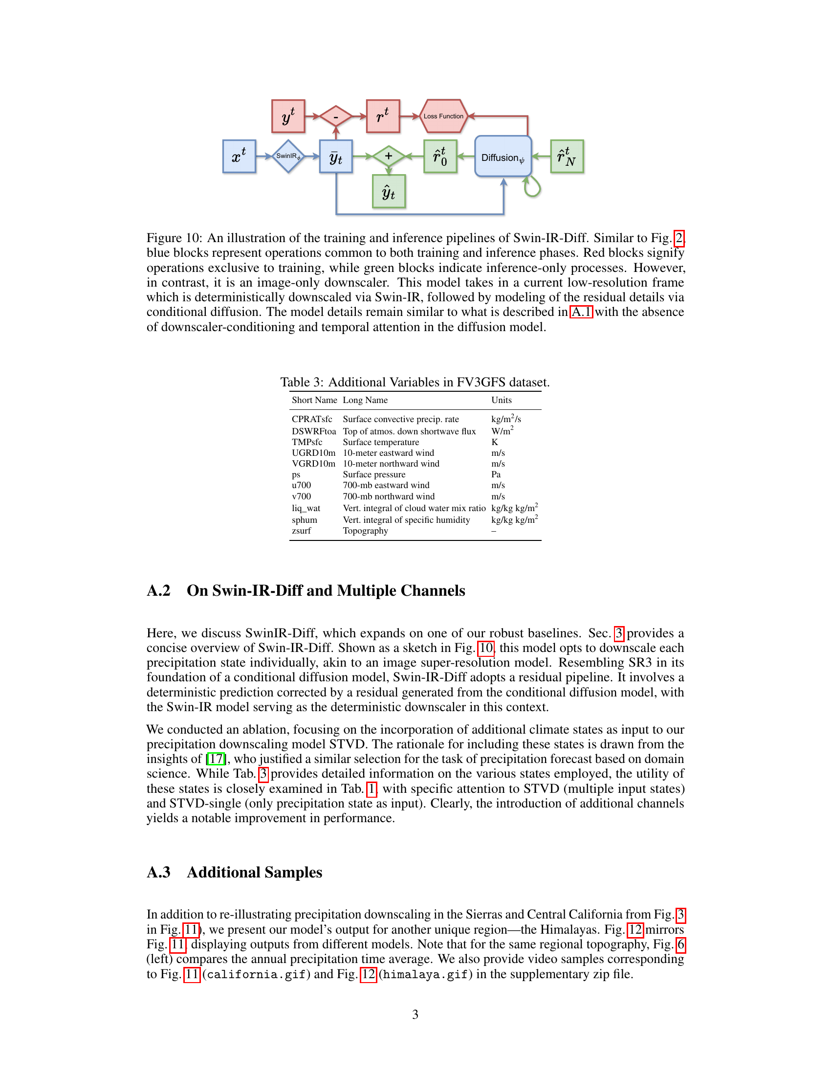
🔼 This figure illustrates the training and inference pipeline of the proposed SpatioTemporal Video Diffusion (STVD) model for precipitation downscaling. It shows how low-resolution precipitation sequences are processed in two main stages. First, a deterministic downscaling module, utilizing spatio-temporal factorized attention, generates an initial high-resolution prediction. Second, a temporally-conditioned diffusion model refines this prediction by modeling the residual errors to capture the high-frequency patterns and noise characteristics present in the high-resolution data. The entire process involves optimizing model parameters jointly during training, incorporating conditional diffusion and factorized attention mechanisms for improved efficiency and accuracy. The figure uses color-coded blocks to distinguish between operations in the training and inference phases.
read the caption
Figure 2: Our model's training and inference pipelines: Blue blocks apply to both phases, red blocks to training only, and green blocks to inference only. It deterministically downscales a low-resolution precipitation sequence using spatio-temporal factorized attention and models residuals with conditional diffusion (with factorized attention). Here, T denotes sequence length and N denotes diffusion steps. The parameters (φ = φ, ψ) are optimized jointly during training. See A.1 for details.
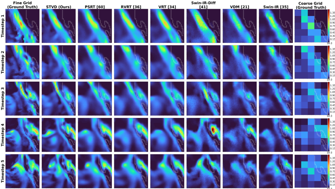
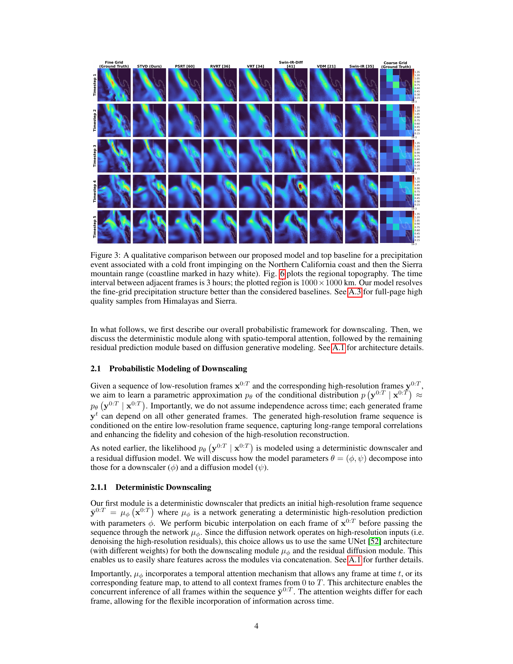
🔼 This figure compares the precipitation prediction of the proposed model (STVD) against other state-of-the-art baselines. It shows a time series of precipitation frames over a 1000x1000km area in Northern California, focusing on a specific precipitation event associated with a cold front. The comparison highlights that STVD better resolves the details of the precipitation than the other models, particularly its high-resolution features.
read the caption
Figure 3: A qualitative comparison between our proposed model and top baseline for a precipitation event associated with a cold front impinging on the Northern California coast and then the Sierra mountain range (coastline marked in hazy white). Fig. 6 plots the regional topography. The time interval between adjacent frames is 3 hours; the plotted region is 1000 × 1000 km. Our model resolves the fine-grid precipitation structure better than the considered baselines. See A.3 for full-page high-quality samples from Himalayas and Sierra.

🔼 This figure shows the trade-off between mean square error (MSE) and percentile error (PE) for different numbers of sampling steps in the SpatioTemporal Video Diffusion (STVD) model. Lower MSE generally indicates better average accuracy, while lower PE signifies better accuracy in capturing extreme precipitation events. The plot reveals a typical inverse relationship: as the number of sampling steps increases, the MSE tends to increase slightly, but the PE decreases significantly, highlighting a balance between average accuracy and the accurate prediction of extreme precipitation events. The inference is performed on the Himalayan region, further detailed in figures 6 and 12 of the paper.
read the caption
Figure 4: Tradeoff between mean square error and percentile error (see Sec. 3). Inference at Himalayan region (see Figs. 6 and 12).

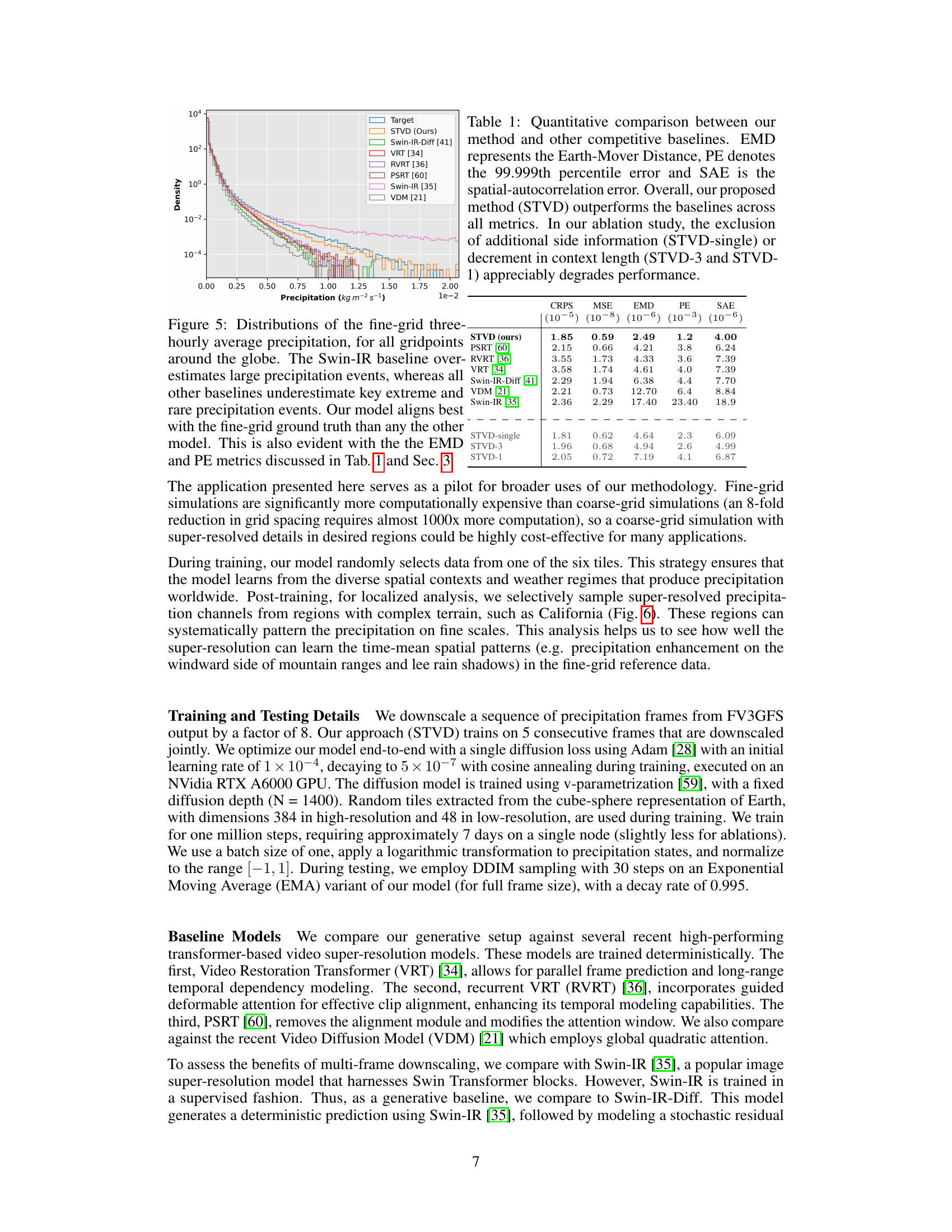
🔼 This figure displays the distribution of fine-grid three-hourly average precipitation across all grid points globally. It compares the distributions generated by the proposed STVD model against six baseline models: Swin-IR, Swin-IR-Diff, VRT, RVRT, PSRT, and VDM. The plot shows that Swin-IR overestimates large precipitation events while the other baselines underestimate them. The STVD model’s distribution is shown to align best with the ground truth distribution.
read the caption
Figure 5: Distributions of the fine-grid three-hourly average precipitation, for all gridpoints around the globe. The Swin-IR baseline over-estimates large precipitation events, whereas all other baselines underestimate key extreme and rare precipitation events. Our model aligns best with the fine-grid ground truth than any the other model. This is also evident with the the EMD and PE metrics discussed in Tab. 1 and Sec. 3.

🔼 This figure shows a comparison of yearly averaged precipitation between the model and ground truth for two different regions: Himalayas and Northern California. The top half of the figure shows the topography and the bottom half shows the precipitation. The left side shows the Himalayas, and the right side shows the California coast. This figure highlights the model’s ability to capture fine details in precipitation patterns that are related to the local topography and are not captured in the coarser ground truth data.
read the caption
Figure 6: Precipitation over two regions (left: Himalayas; right: Northern California coast, same region as Fig. 3), averaged across a year, for our STVD model and the ground-truth. For each half, the topography of the region is shown in the corresponding top-left whereas the predicted annual average is shown in the corresponding bottom-right. Annually-averaged precipitation is an important indicator of water availability in a region. STVD successfully captures many details of the precipitation that are tied to local topography and are too fine to be resolved the coarse-grid data.
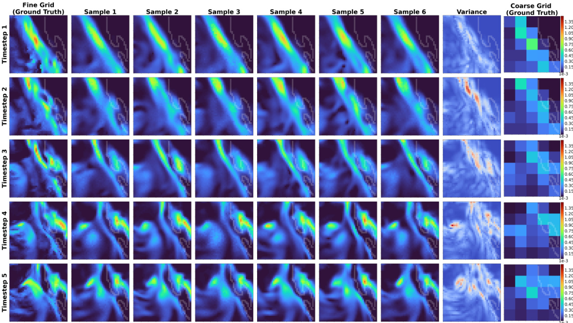
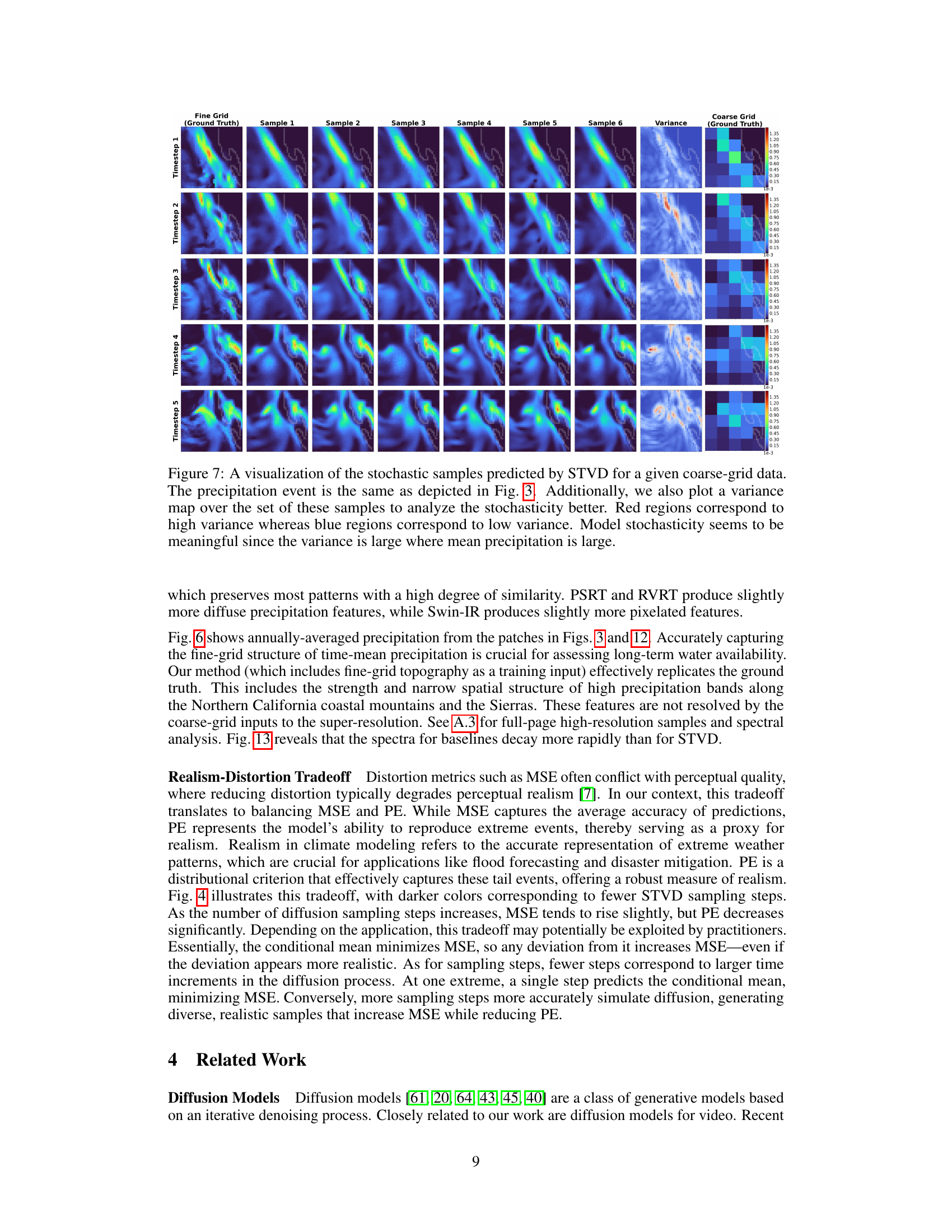
🔼 This figure visualizes the stochasticity of the STVD model by showing multiple samples generated from the same coarse-grid input. The samples show variations, especially in areas with higher precipitation amounts, indicating that the model’s stochasticity is not random noise but reflects the inherent uncertainty in predicting precipitation.
read the caption
Figure 7: A visualization of the stochastic samples predicted by STVD for a given coarse-grid data. The precipitation event is the same as depicted in Fig. 3. Additionally, we also plot a variance map over the set of these samples to analyze the stochasticity better. Red regions correspond to high variance whereas blue regions correspond to low variance. Model stochasticity seems to be meaningful since the variance is large where mean precipitation is large.
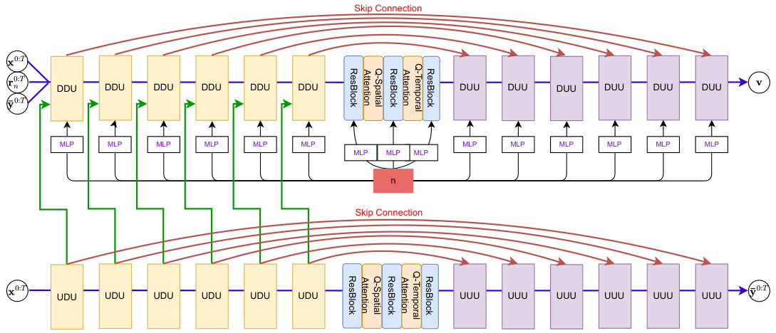
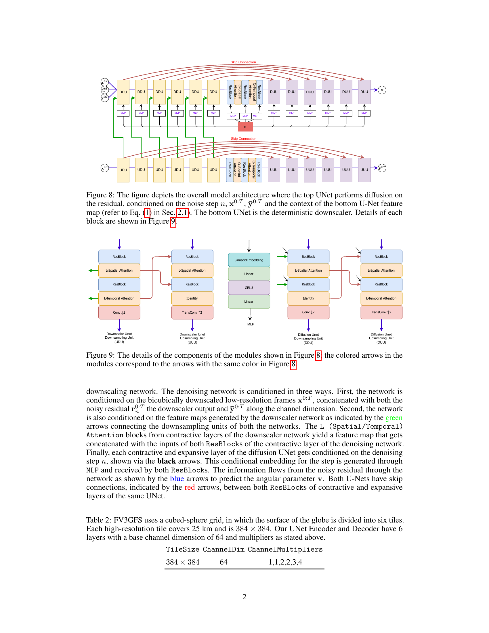
🔼 This figure shows the overall architecture of the proposed model. It’s composed of two UNets: a top UNet for diffusion on the residual and a bottom UNet acting as a deterministic downscaler. The top UNet conditions on the noise step, the low-resolution frames, the initial prediction, and the feature maps from the bottom UNet. The bottom UNet processes low-resolution frames to produce an initial precipitation prediction.
read the caption
Figure 8: The figure depicts the overall model architecture where the top UNet performs diffusion on the residual, conditioned on the noise step n, x0:T, ŷ0:T and the context of the bottom U-Net feature map (refer to Eq. (1) in Sec. 2.1). The bottom UNet is the deterministic downscaler. Details of each block are shown in Figure 9.

🔼 This figure illustrates the overall architecture of the proposed model. The model consists of two UNets: a top UNet which performs diffusion on the residual and a bottom UNet which acts as a deterministic downscaler. The top UNet conditions on three things: the noise step n, the low-resolution sequence x0:T, the downscaler output ŷ0:T. The bottom UNet takes in the low-resolution sequence and outputs the deterministic prediction. Figure 9 further details each individual block shown here.
read the caption
Figure 8: The figure depicts the overall model architecture where the top UNet performs diffusion on the residual, conditioned on the noise step n, x0:T, ŷ0:T and the context of the bottom U-Net feature map (refer to Eq. (1) in Sec. 2.1). The bottom UNet is the deterministic downscaler. Details of each block are shown in Figure 9.

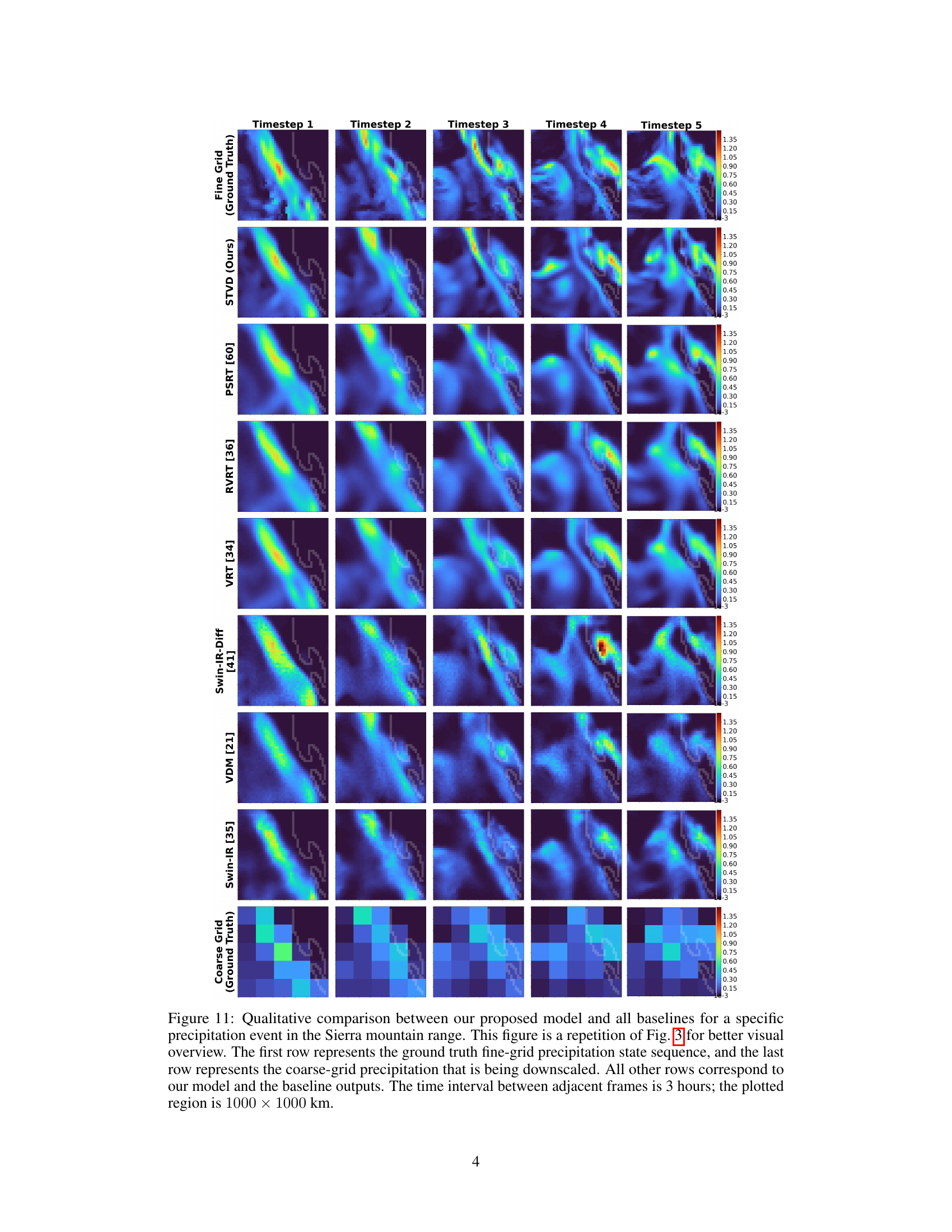
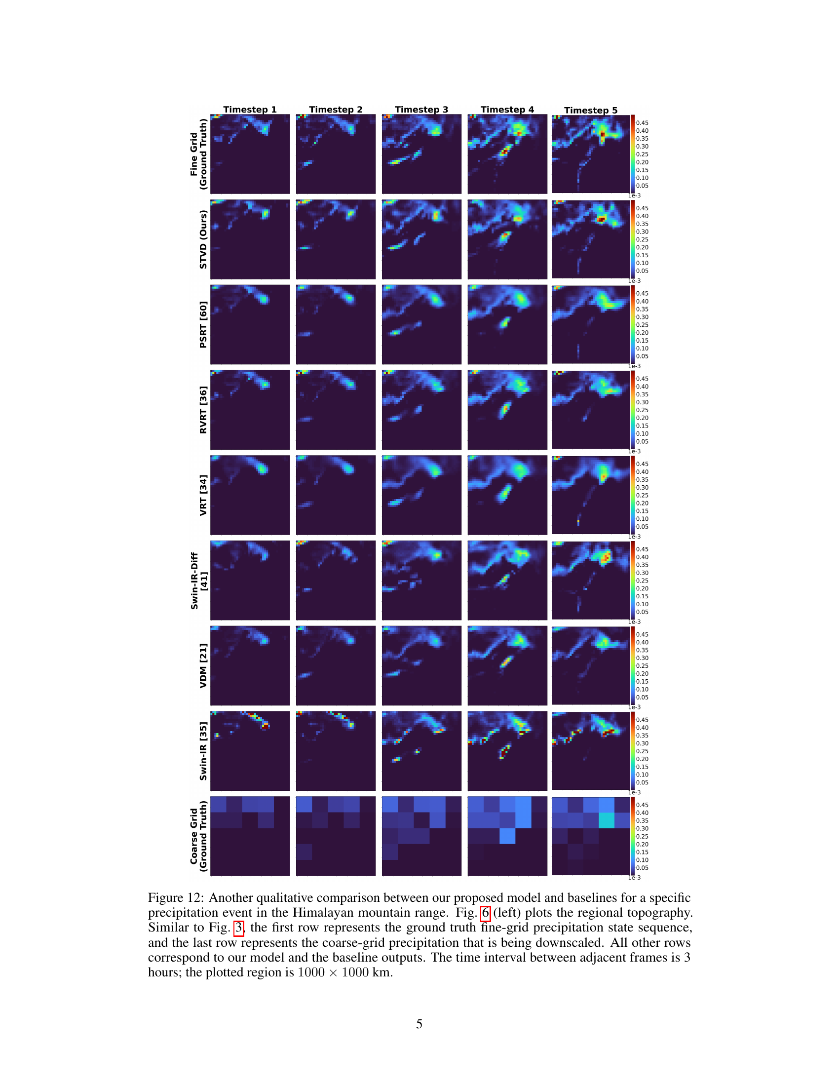
🔼 This figure compares the performance of the proposed model (STVD) against six state-of-the-art baselines in downscaling precipitation data. It shows a specific precipitation event in the Sierra Nevada mountain range over a 5 timestep period. Each row shows the results from a different model, with the top row being ground truth and the bottom row showing the original coarse-resolution input. The figure highlights the ability of the proposed model to better capture fine-grained details in the precipitation patterns compared to existing methods.
read the caption
Figure 11: Qualitative comparison between our proposed model and all baselines for a specific precipitation event in the Sierra mountain range. This figure is a repetition of Fig. 3 for better visual overview. The first row represents the ground truth fine-grid precipitation state sequence, and the last row represents the coarse-grid precipitation that is being downscaled. All other rows correspond to our model and the baseline outputs. The time interval between adjacent frames is 3 hours; the plotted region is 1000 × 1000 km.

🔼 This figure compares the results of the proposed model (STVD) against six state-of-the-art baselines in a specific precipitation event in the Sierra Nevada mountain range. It shows a time-series of precipitation frames, where the first row displays the ground truth at high resolution, the last row displays the low-resolution input, and the rows in-between show the outputs of the different models at high resolution. This visualization provides a qualitative comparison of model performance in terms of detail and accuracy in capturing precipitation patterns.
read the caption
Figure 11: Qualitative comparison between our proposed model and all baselines for a specific precipitation event in the Sierra mountain range. This figure is a repetition of Fig. 3 for better visual overview. The first row represents the ground truth fine-grid precipitation state sequence, and the last row represents the coarse-grid precipitation that is being downscaled. All other rows correspond to our model and the baseline outputs. The time interval between adjacent frames is 3 hours; the plotted region is 1000 × 1000 km.
🔼 This figure compares the qualitative results of the proposed model (STVD) against six baselines for a precipitation event in the Sierra Nevada mountain range. It shows a time series of precipitation maps, with the ground truth (fine-resolution) at the top and the low-resolution input at the bottom. The middle rows show the results of different models, demonstrating the ability of STVD to better capture fine details compared to the baselines.
read the caption
Figure 11: Qualitative comparison between our proposed model and all baselines for a specific precipitation event in the Sierra mountain range. This figure is a repetition of Fig. 3 for better visual overview. The first row represents the ground truth fine-grid precipitation state sequence, and the last row represents the coarse-grid precipitation that is being downscaled. All other rows correspond to our model and the baseline outputs. The time interval between adjacent frames is 3 hours; the plotted region is 1000 × 1000 km.

🔼 This figure visualizes the average temporal attention weights computed across the entire validation dataset and all attention heads within the bottleneck layer of the deterministic downscaler component of the proposed model. The visualization is a 5x5 heatmap, where each cell represents the attention weight between two temporal positions in the sequence (T1-T5). Brighter colors indicate stronger attention weights. The figure demonstrates that attention weights decay as the temporal distance between positions increases, reflecting the expected behavior of a model that prioritizes nearby temporal information. For example, the highest attention weights are observed for a frame and its immediate neighbors.
read the caption
Figure 14: A visualization of the temporal attention weights averaged over the entire validation set and attention heads for the bottleneck layer of the deterministic downscaler. T1 - T5 denotes the temporal sequence. The weights evidently decay as a function of temporal distance which makes physical sense. For example, feature map at position T2 attends the most towards itself along with immediate temporal neighbors at T1 and T3. Lighter colors correspond to larger weight.
More on tables

🔼 This table presents a quantitative comparison of the proposed SpatioTemporal Video Diffusion (STVD) model against six state-of-the-art baselines using various metrics. The metrics include Earth Mover’s Distance (EMD), 99.999th percentile error (PE), and spatial autocorrelation error (SAE). The results demonstrate that STVD outperforms all baselines. Ablation studies, removing additional information or reducing context length, show a significant decrease in performance, highlighting the importance of these factors in STVD’s success.
read the caption
Table 1: Quantitative comparison between our method and other competitive baselines. EMD represents the Earth-Mover Distance, PE denotes the 99.999th percentile error and SAE is the spatial-autocorrelation error. Overall, our proposed method (STVD) outperforms the baselines across all metrics. In our ablation study, the exclusion of additional side information (STVD-single) or decrement in context length (STVD-3 and STVD-1) appreciably degrades performance.

🔼 This table presents a quantitative comparison of the proposed SpatioTemporal Video Diffusion (STVD) model against six other state-of-the-art baselines across multiple evaluation metrics. The metrics used include the Earth Mover’s Distance (EMD), 99.999th percentile error (PE), and spatial autocorrelation error (SAE). The results demonstrate that STVD outperforms all baselines. Additionally, an ablation study shows that removing additional information or reducing the temporal context significantly reduces the performance of the model.
read the caption
Table 1: Quantitative comparison between our method and other competitive baselines. EMD represents the Earth-Mover Distance, PE denotes the 99.999th percentile error and SAE is the spatial-autocorrelation error. Overall, our proposed method (STVD) outperforms the baselines across all metrics. In our ablation study, the exclusion of additional side information (STVD-single) or decrement in context length (STVD-3 and STVD-1) appreciably degrades performance.
Full paper#
