Finding good policies in average-reward Markov Decision Processes without prior knowledge

↗ OpenReview ↗ NeurIPS Homepage ↗ Chat

TL;DR

#

Key Takeaways

#

Why does it matter?

#

This paper is crucial because it addresses the challenge of finding optimal policies in average-reward Markov Decision Processes (MDPs) without prior knowledge of the MDP’s complexity—a significant limitation of existing methods. It presents novel algorithms with near-optimal sample complexities and offers valuable insights into the inherent hardness of the online setting, shaping future research directions in reinforcement learning.

Visual Insights

#

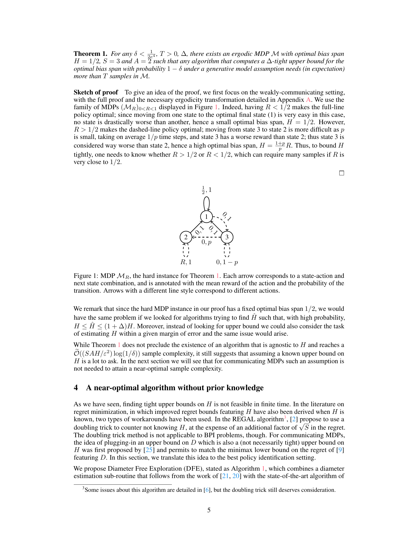
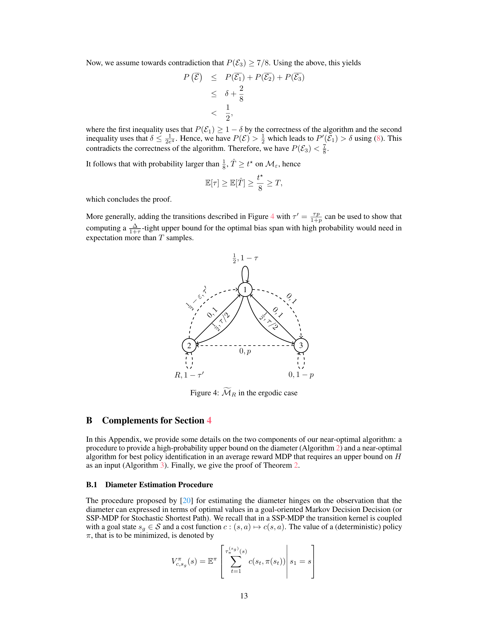
This figure shows a Markov Decision Process (MDP) used to prove Theorem 1, which states that estimating the optimal bias span H requires an arbitrarily large number of samples. The MDP has three states (1, 2, 3) and two actions for each state. The solid lines represent one action and the dashed lines represent the other action, which have different reward and transition probabilities. The parameter R determines the optimal policy and bias span. If R < 1/2, the solid-line policy is optimal and the bias span is small. If R > 1/2, the dashed-line policy is optimal and the bias span is large. The difficulty of accurately estimating H arises when R is very close to 1/2, as many samples are needed to distinguish between the two cases.

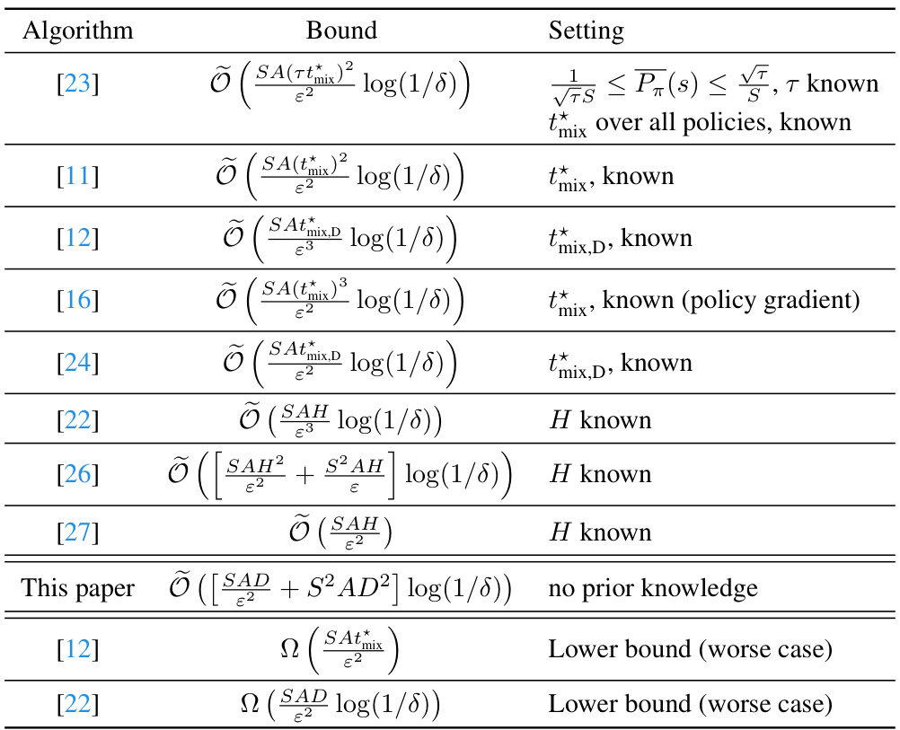
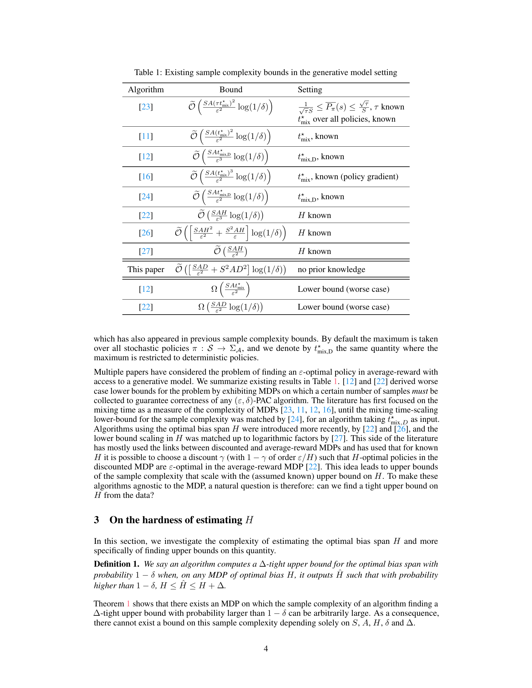
This table summarizes existing sample complexity bounds in the literature for the problem of finding an ε-optimal policy in average-reward Markov Decision Processes (MDPs) using a generative model. It compares different algorithms and their sample complexity bounds, highlighting the influence of various complexity measures, such as the mixing time (t_mix), diameter (D), and optimal bias span (H). The table also includes lower bounds which demonstrate the inherent complexity of the problem. The ‘Setting’ column specifies which parameters are assumed to be known to the algorithm.

In-depth insights

#

Policy ID Limits

#

The heading ‘Policy ID Limits’ suggests an exploration of inherent constraints in policy identification methods within the context of reinforcement learning or Markov Decision Processes. A thoughtful analysis would delve into computational complexity, examining whether the time or resources required for accurate policy identification scale polynomially or exponentially with problem size (state and action space dimensions). Sample complexity, the minimum number of interactions needed to identify an optimal or near-optimal policy, is another critical aspect. The analysis should investigate lower and upper bounds for sample complexity, ideally demonstrating near-optimality of proposed algorithms. A discussion of the role of model assumptions is essential; identifying whether the algorithms rely on a fully generative model or a more limited setting (e.g., online learning) significantly affects feasibility and performance. Finally, the exploration of various complexity measures for MDPs, beyond simple state and action space dimensions, and their impact on policy identification limits is crucial; the analysis could touch upon concepts such as diameter, bias span, or mixing time. Prior knowledge about the MDP could influence the limitations; ideally, the study should contrast the performance between algorithms that require and those that do not require such prior knowledge.

Estimating H

#

The estimation of the optimal bias span, H, presents a significant challenge in average-reward Markov Decision Processes (MDPs). Existing algorithms for policy identification often rely on prior knowledge of H or a readily available upper bound, which limits their applicability and practicality in real-world scenarios. The theoretical analysis reveals that directly estimating H is computationally intractable, requiring a sample complexity that is not polynomially bounded by the relevant parameters (S, A, H, δ, and Δ). This difficulty stems from the inherent sensitivity of H to subtle changes in the MDP’s transition dynamics and reward structure, making it extremely challenging to learn from limited samples. Therefore, alternative strategies that bypass explicit H estimation are crucial. Rather than focusing on precisely estimating H, research is moving toward using more readily estimable quantities, such as the diameter D (which is an upper bound for H), for policy identification. This approach helps maintain near-optimal sample complexity while eliminating the dependence on prior knowledge of H.

Diameter Free Exploration

#

The proposed “Diameter Free Exploration” algorithm offers a novel approach to solving average-reward Markov Decision Processes (MDPs) without prior knowledge of the MDP’s structure. Instead of relying on the often-hard-to-estimate optimal bias span (H), it leverages the diameter (D) as a readily available complexity measure. This is a significant contribution because estimating H is computationally challenging and often intractable. The algorithm cleverly combines a procedure for estimating D with an existing policy identification algorithm to achieve a near-optimal sample complexity in the regime of small epsilon (error tolerance). The elimination of prior knowledge about H makes the algorithm more practical and broadly applicable. While the algorithm’s sample complexity is nearly optimal in the generative model setting, its online variant introduces an additional factor related to the diameter, leading to a slightly higher complexity. Future research directions include exploring more adaptive sampling and stopping rules to further improve the online algorithm’s efficiency and potentially close the gap between its performance and existing theoretical lower bounds.

Online Hardness

#

The section on “Online Hardness” would likely explore the inherent challenges of solving average-reward Markov Decision Processes (MDPs) in an online setting, where the agent interacts with the environment sequentially and without prior knowledge of the environment’s dynamics. A key difficulty is the trade-off between exploration and exploitation: the agent must balance the need to learn about the environment (exploration) with the need to act optimally based on its current knowledge (exploitation). Unlike the generative model setting where the agent can sample from any state-action pair, the online setting presents a more limited information acquisition process. The sample complexity required for effective learning is a major focus; demonstrating that achieving polynomial sample complexity dependent on the optimal bias span (H) isn’t always possible, is a significant contribution. This implies that algorithms agnostic to H are necessary for the online setting, necessitating new techniques for online policy identification that overcome the limitations imposed by sequential information acquisition and the inherent uncertainty in the system dynamics.

Adaptive Rules

#

Adaptive rules in reinforcement learning aim to dynamically adjust learning parameters based on observed data, improving efficiency and performance. Contextual adaptation, responding to the specific challenges of a given state or environment, is key. This contrasts with static rules, which maintain fixed parameters regardless of the situation. Data-driven adaptation uses statistical measures, such as confidence intervals or error estimates, to inform parameter adjustments. This approach allows the agent to balance exploration and exploitation, efficiently learning optimal policies while mitigating risks associated with uncertainty. Reward-based adaptation uses observed rewards to guide the learning process, directing exploration towards more promising actions. Adaptive sampling techniques, which determine the number or type of samples taken in response to prior outcomes, further enhance the effectiveness of adaptive learning. Successful adaptive rules require careful consideration of the balance between responsiveness and stability; excessively reactive rules can lead to instability, while overly cautious rules may miss opportunities for faster learning. Effective implementation often involves balancing these competing priorities, achieving both flexibility and efficiency in the learning process.

More visual insights

#

More on figures

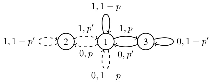
This figure shows a Markov Decision Process (MDP) used in Theorem 1 to demonstrate the hardness of estimating the optimal bias span H. The MDP has three states (1, 2, 3) and two actions for each state, represented by solid and dashed arrows. The numbers on the arrows indicate the reward obtained and the probability of transitioning to the next state when that action is chosen. The structure of the MDP is designed such that depending on the exact value of a parameter R, either the solid lines or the dashed lines will result in an optimal policy. However, R’s value is close to 1/2 (the transition point between the two optimal policies), making it difficult to determine the optimal policy (and thus estimate H accurately) with a limited number of samples.

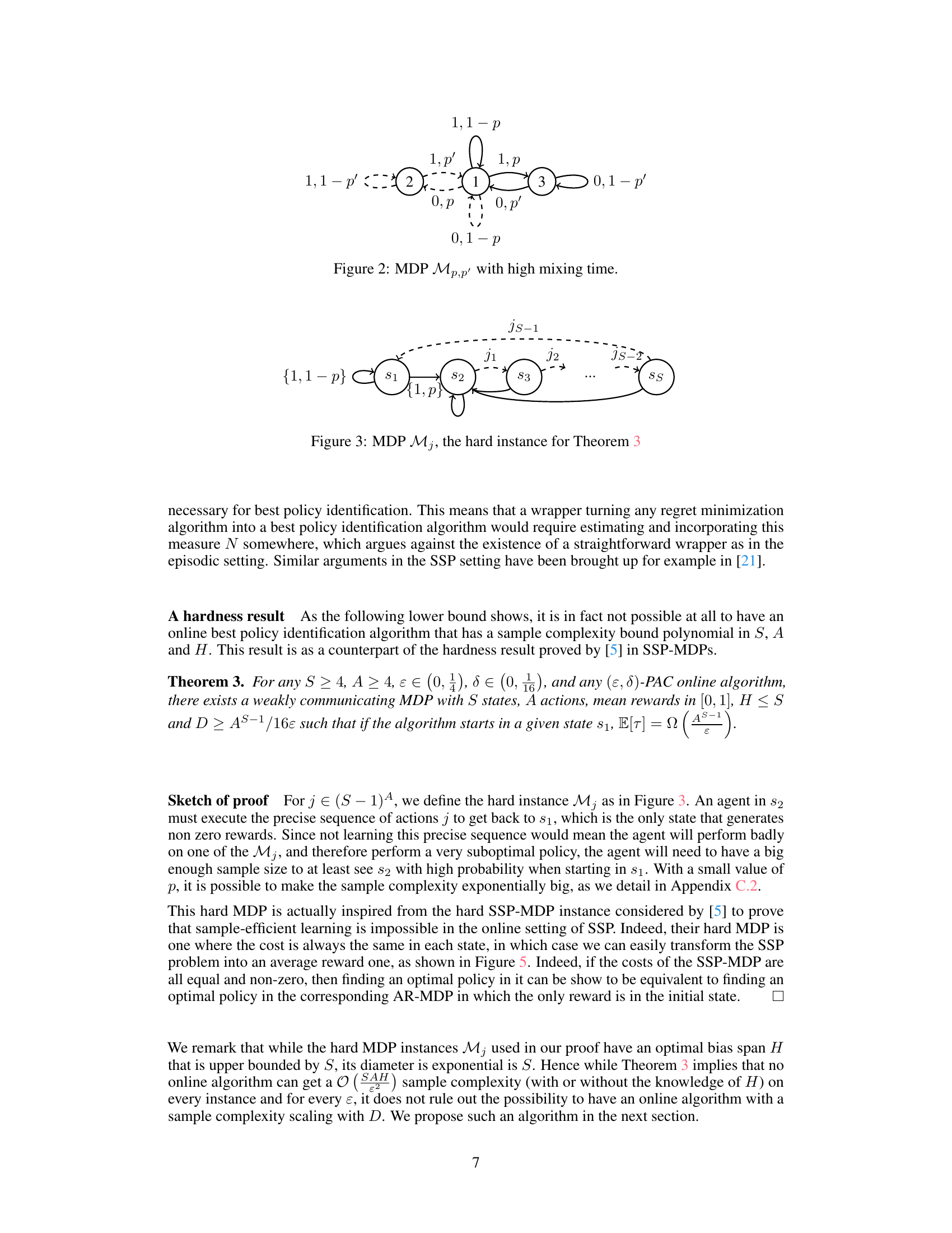
This figure shows a Markov Decision Process (MDP) used to prove Theorem 3, which states that there is no online algorithm with sample complexity polynomial in S, A, and H for best policy identification. The MDP has S states (s1, s2, …, sS) and A actions. The transition probabilities are such that reaching state s2 from s1 requires a specific sequence of actions. The reward is 1 only in state s1. This construction is used to show that any algorithm must explore the state space sufficiently to encounter the high-reward state s1 and learn the optimal sequence of actions.

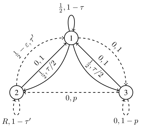
This figure shows a Markov Decision Process (MDP) that is used to prove Theorem 1 in the paper. The MDP is designed to be difficult to estimate the optimal bias span, H. The MDP has three states (1, 2, and 3) and two actions. Depending on the parameter R (where 0 < R < 1), either a solid line or a dashed line policy is optimal. The complexity arises because if R is close to 1/2, it requires many samples to determine whether R is greater than or less than 1/2, significantly impacting the complexity of estimating H.

This figure shows a Markov Decision Process (MDP) used in the proof of Theorem 1 to demonstrate that estimating the optimal bias span H can be computationally hard. The MDP has three states (1, 2, 3) and two actions for each state. The actions are represented by solid and dashed arrows, with different transition probabilities and rewards for each. The parameter R is used to control whether the optimal policy is the dashed or solid line policy. This is critical because when R is close to 0.5, a very large number of samples are required to distinguish between R < 0.5 and R > 0.5.

This figure shows a Markov Decision Process (MDP) used in the proof of Theorem 1. The MDP has three states and two actions. The transitions and rewards are controlled by a parameter R. The figure demonstrates how the optimal policy, and therefore the optimal bias span, changes depending on whether R is less than or greater than 1/2. This property makes it difficult to estimate the optimal bias span H efficiently, which is central to the theorem’s proof.

Full paper

#