↗ OpenReview ↗ NeurIPS Homepage ↗ Chat
TL;DR#
Time series forecasting is hindered by limited data and privacy issues. Existing methods struggle to share knowledge across domains efficiently while respecting data ownership. This limits the development of generalizable Foundation Models (FMs).
TIME-FFM innovatively addresses these by transforming time series into text, using pre-trained Language Models to extract temporal patterns. A prompt adaptation module personalizes the model for different domains, and a federated learning strategy enables distributed training without raw data sharing. Extensive experiments demonstrate that TIME-FFM surpasses existing methods in accuracy and efficiency, especially in low-data scenarios.
Key Takeaways#
Why does it matter?#
This paper is crucial because it addresses the scarcity of data in time series forecasting by proposing TIME-FFM, a novel Federated Foundation Model. This model leverages pre-trained Language Models and a personalized federated training strategy to achieve superior few-shot and zero-shot forecasting performance, while respecting data privacy. Its impact extends to various real-world applications where data sharing is limited, such as healthcare and finance, opening up new avenues for research and development in the field.
Visual Insights#

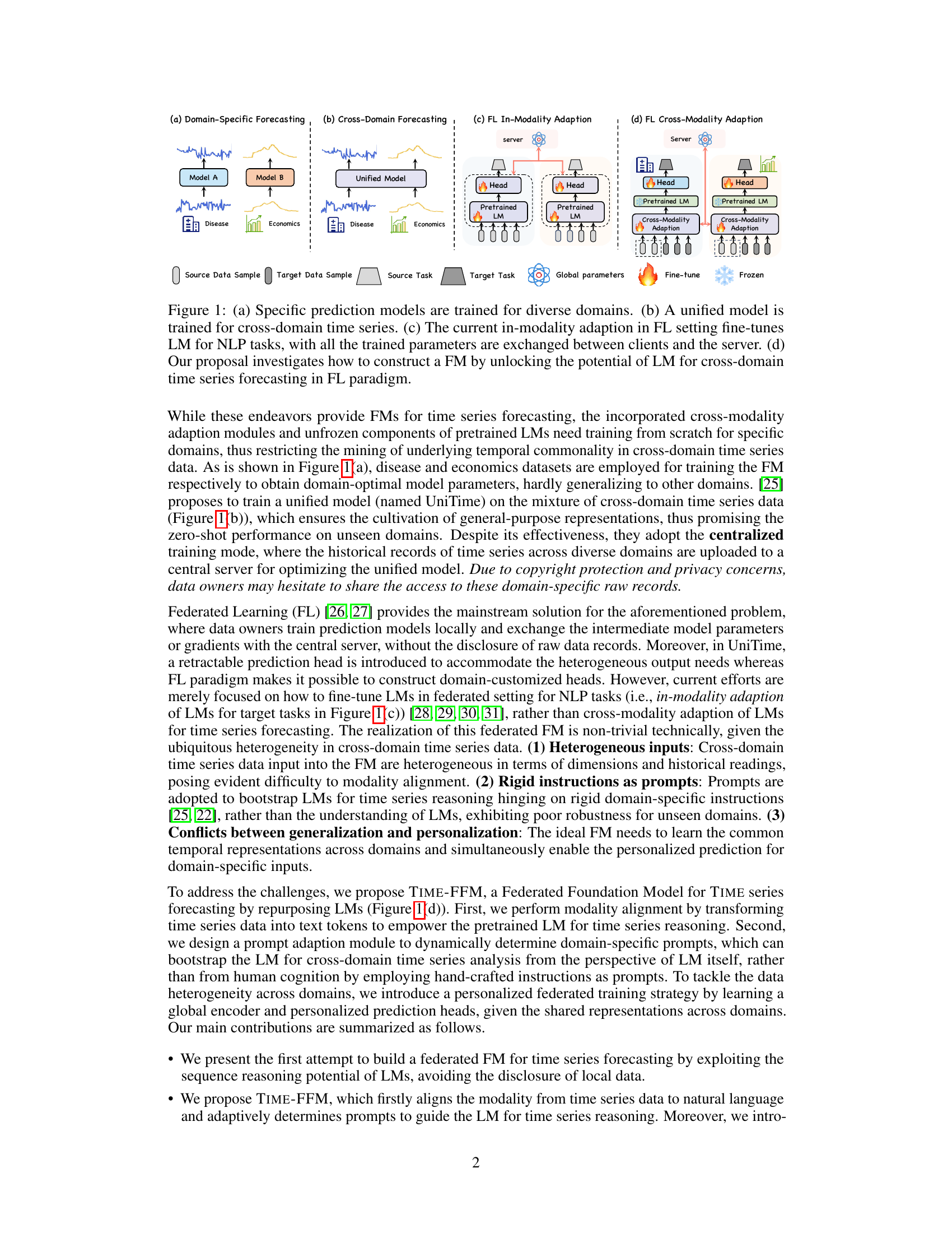
This figure illustrates four different approaches to time series forecasting. (a) shows the traditional approach of training separate models for each domain. (b) presents a unified model trained on data from multiple domains. (c) depicts the current federated learning (FL) approach, where language models (LMs) are fine-tuned for specific tasks, and parameters are exchanged between clients and a central server. (d) introduces the proposed approach, TIME-FFM, which leverages pretrained LMs for cross-domain time series forecasting in a federated learning setting.
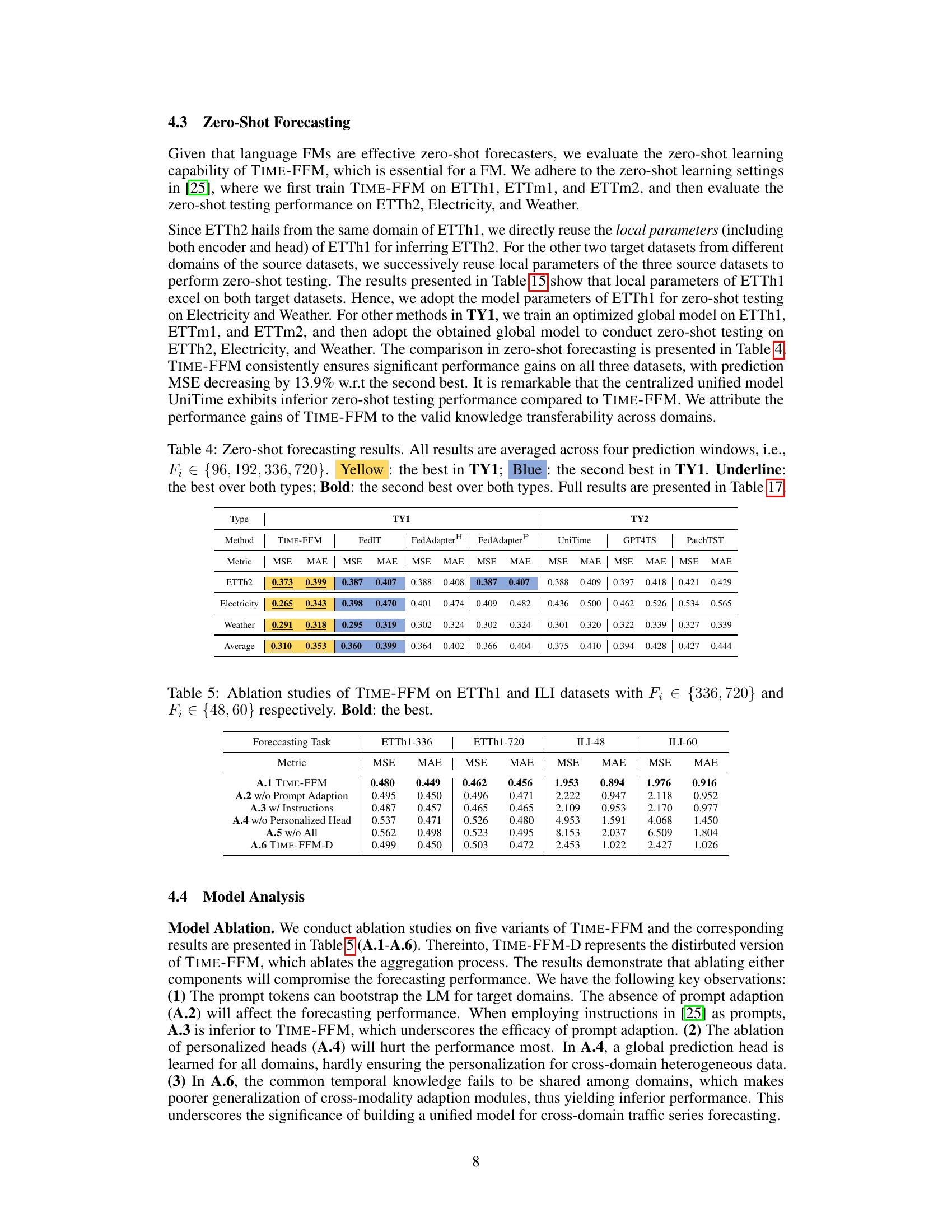
This table presents a comparison of forecasting performance metrics (MSE and MAE) across multiple methods categorized into three types (TY1, TY2, TY3). Each method’s performance is averaged over four different prediction window lengths. Color-coding highlights the best and second-best performing methods within TY1, while underlining and bolding indicate the best and second-best methods across all three types.
In-depth insights#
Federated LM for TS#
A federated learning approach using large language models (LLMs) for time series (TS) forecasting offers a compelling solution to address data scarcity and privacy concerns in the TS domain. Federated learning allows multiple entities to collaboratively train an LLM on their respective local TS datasets without directly sharing the raw data. This preserves data privacy and enables the construction of a more robust and generalized LLM for TS forecasting. The use of LLMs is particularly promising because their inherent ability to capture complex patterns and relationships in sequential data translates well to the challenges of TS prediction. However, challenges include modality alignment (transforming time series into a format suitable for LLMs), prompt engineering (designing effective prompts that guide the LLM’s reasoning), and federated training strategies that ensure effective global model learning while accommodating domain-specific characteristics. Successful implementation requires careful consideration of these aspects to balance generalization and personalization across diverse datasets.
Cross-Domain TS-FM#
A Cross-Domain TS-FM (Time Series Foundation Model) aims to address the limitations of traditional time series forecasting models by building a single model capable of handling diverse datasets from various domains. This contrasts with conventional approaches which train separate models for each domain, leading to a lack of generalization and inefficiency. A key challenge lies in handling the heterogeneity of data from different domains, requiring robust techniques for data preprocessing and model adaptation. A successful Cross-Domain TS-FM should leverage shared temporal patterns across domains, using techniques like transfer learning or multi-task learning to improve performance and reduce the need for extensive training data per domain. Federated learning may play a crucial role in enabling the construction of such models by allowing training on decentralized data while maintaining privacy. Finally, careful consideration of model architecture, including potentially using transformer-based models, is critical for capturing long-range dependencies and relationships in time series data effectively.
Prompt Adaptation#
Prompt adaptation, in the context of large language models (LLMs) for time series forecasting, is a crucial technique to effectively leverage the power of pre-trained models for diverse downstream tasks. The core idea is to dynamically generate prompts rather than using static, pre-defined instructions, allowing the LMs to better understand and reason about the specific characteristics of the time series data. This approach addresses the challenge of data heterogeneity across domains by enabling the model to adapt its reasoning process to the unique nuances of each dataset. Adaptive prompt generation improves the model’s ability to learn common temporal representations and simultaneously enables personalized predictions. This adaptability is particularly useful in the context of federated learning, where the model needs to perform well across numerous, potentially heterogeneous, datasets without direct access to their raw data. The effectiveness of prompt adaptation ultimately relies on the ability of the LMs to learn and generalize across domains, capitalizing on shared temporal patterns while maintaining task-specific personalization.
Personalized FL#
In the context of federated learning (FL), personalization is crucial because global models trained on aggregated data from diverse clients often fail to capture individual client characteristics. A personalized FL approach, therefore, aims to tailor models to each client’s unique data distribution while still leveraging the benefits of collaborative training. This typically involves learning a shared global model that captures common patterns across clients and combining it with client-specific components (e.g., local prediction heads) that adjust the model to individual needs. This balance between global knowledge sharing and individual model adaptation is key to effectively personalizing FL, which can lead to improved accuracy and reduced communication overhead. Federated personalization techniques must address data heterogeneity, since clients may not have similar features, sample sizes, or data quality. This may involve techniques like domain adaptation or personalized loss functions, to ensure effective model training on diverse datasets.
Few-shot Forecasting#
The section ‘Few-shot Forecasting’ in this research paper explores the model’s ability to perform accurate time series forecasting with limited training data. This is a crucial capability for real-world applications where obtaining large, labeled datasets is often expensive or impractical. The experiments likely involved training the model on a small subset of the available data and then evaluating its performance on unseen data. Key findings likely demonstrate the effectiveness of the proposed method in achieving competitive results with limited data compared to existing methods. This highlights a significant advantage in scenarios with data scarcity, such as new domains or rare events. The results likely showcase the model’s generalization ability, and a comparison against existing few-shot learning techniques in time series would be important. Robustness against noisy or incomplete data is another factor that would likely be discussed in this context, and specific details about the experimental setup (e.g., the percentage of data used for training, evaluation metrics) would be necessary to gain a complete understanding.
More visual insights#
More on figures
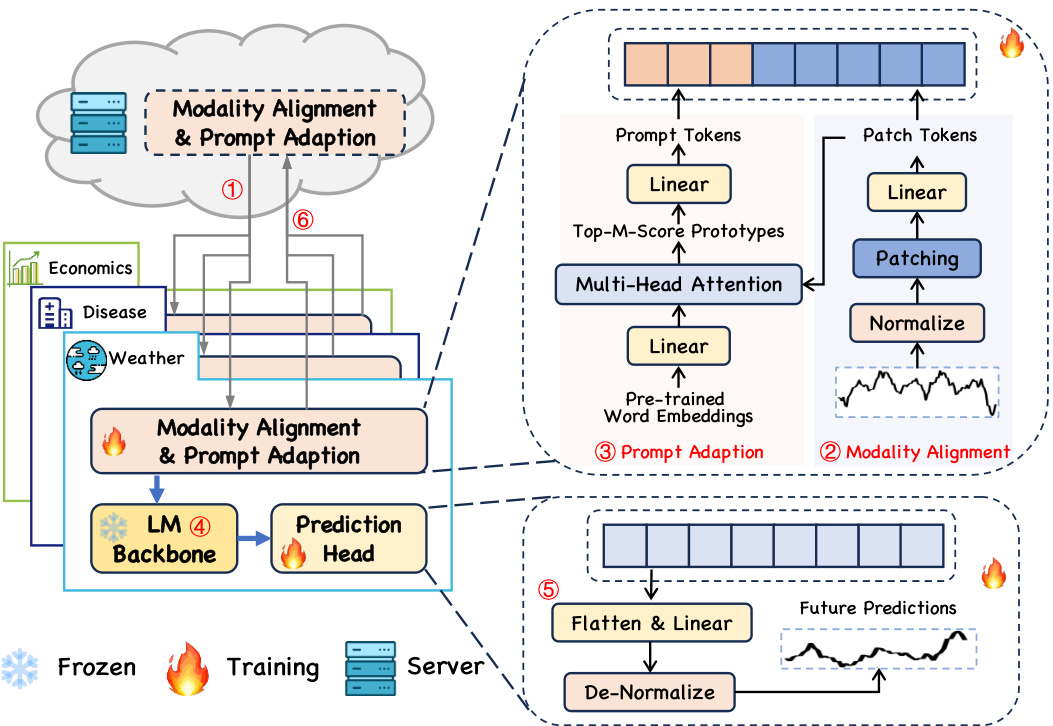
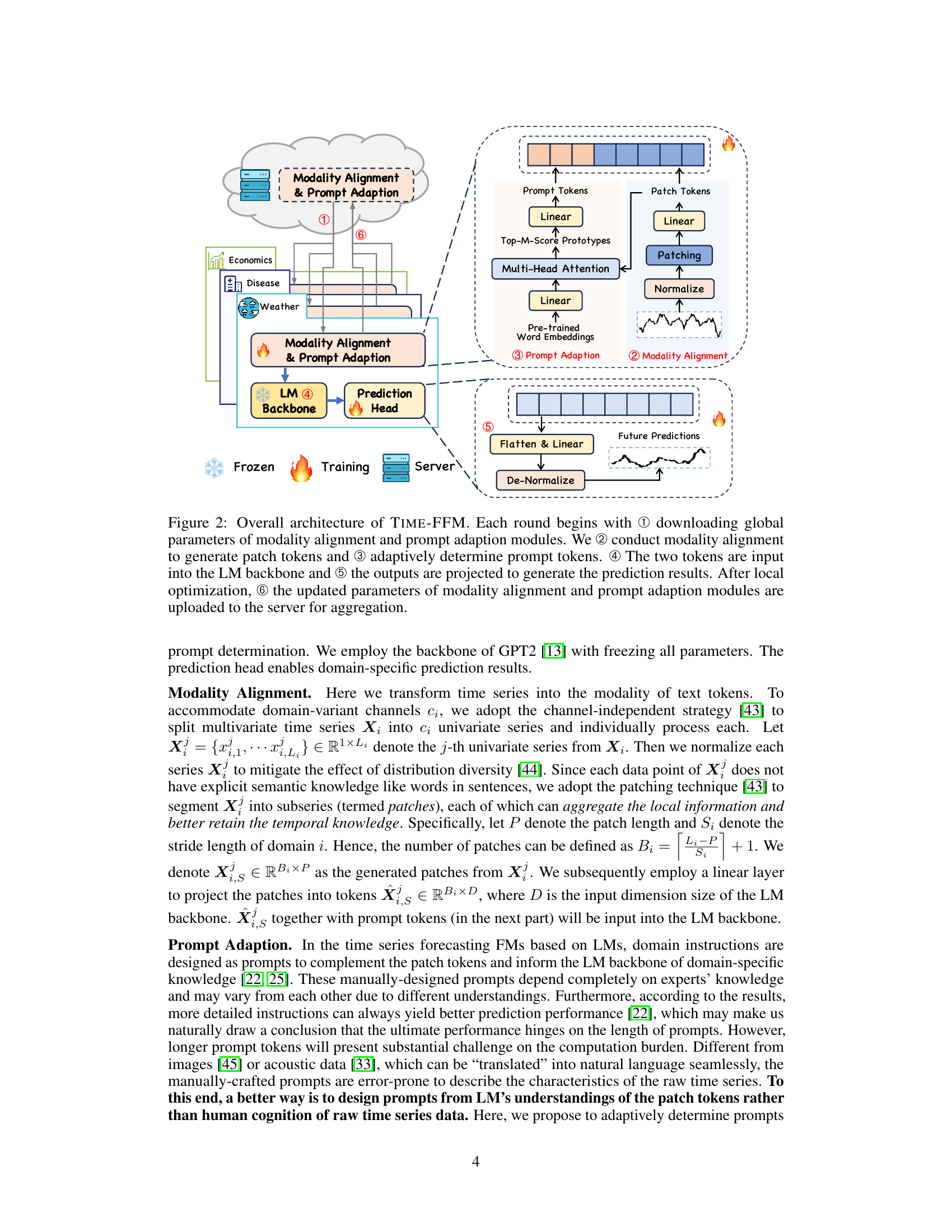
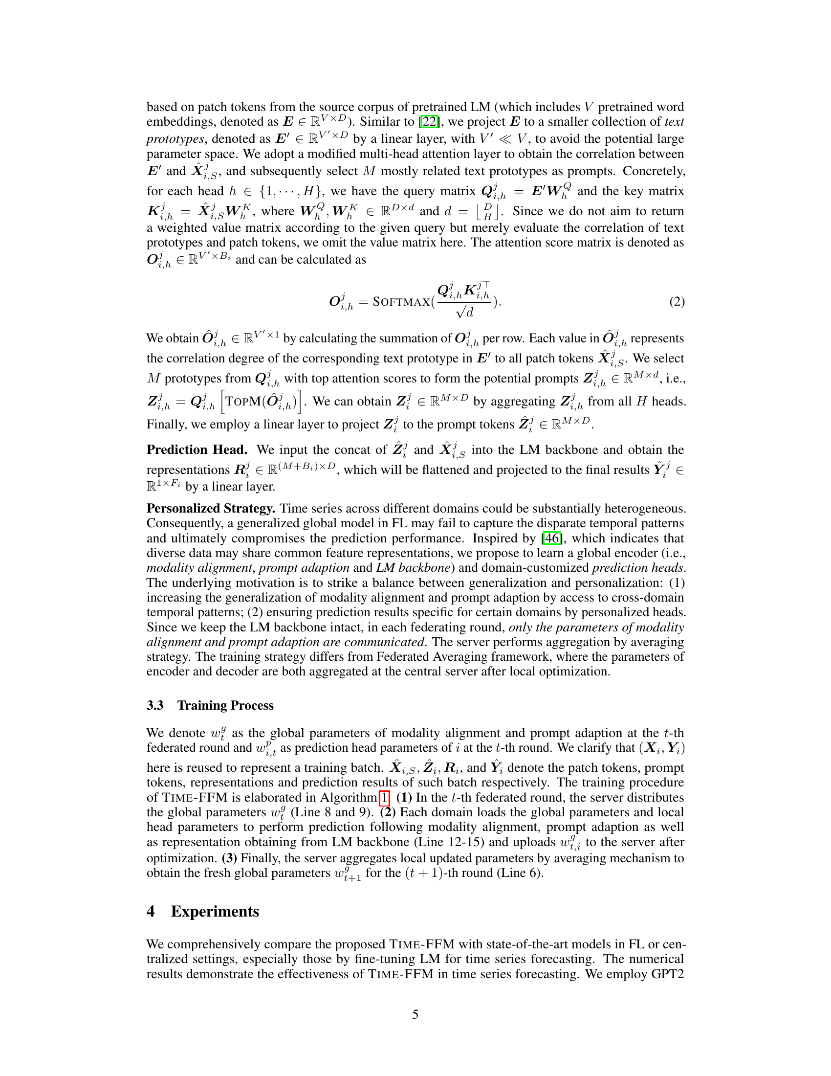
The figure illustrates the overall architecture of the TIME-FFM model. It shows how the model processes time-series data in a federated learning setting, transforming it into a text-based representation using modality alignment and prompt adaption modules. These transformed data are then fed into a pre-trained language model (LM) backbone. The output from the LM is subsequently used to generate predictions, which are then fine-tuned using personalized prediction heads. The process involves the exchange of parameters between local clients and the central server in a federated manner.
This figure illustrates the overall architecture of the TIME-FFM model, highlighting the interaction between clients and server during the federated learning process. The model takes time series data as input and transforms it into text tokens using a modality alignment module. A prompt adaption module then generates domain-specific prompts. These tokens are fed into a pre-trained LM backbone, and the resulting outputs are used to make predictions. The process is iterative, with updates being aggregated on the server after local optimization on each client.

This figure illustrates the overall architecture of the TIME-FFM model, highlighting the different stages involved in each round of federated learning. It shows how global parameters are downloaded, modality alignment and prompt adaption are performed, and how the resulting tokens are fed into the LM backbone for prediction. Finally, it illustrates how the updated parameters are uploaded to the server for aggregation.
More on tables
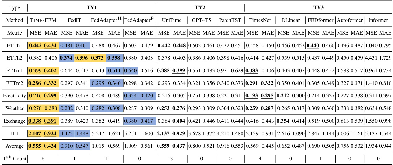
This table presents a comparison of the forecasting performance of TIME-FFM against several other methods across eight benchmark datasets. The metrics used are Mean Squared Error (MSE) and Mean Absolute Error (MAE). The methods are categorized into three types: federated fine-tuning methods (TY1), across-dataset centralized methods (TY2), and dataset-specific centralized methods (TY3). The table highlights the best and second-best performing methods within each category and overall.
This table presents a comparison of forecasting performance across various methods categorized into three types (TY1, TY2, TY3). The metrics used are MSE (Mean Squared Error) and MAE (Mean Absolute Error), averaged over four prediction window lengths for most datasets (except ILI). The table highlights the best (Yellow) and second best (Blue) performing methods within TY1 (Federated fine-tuning methods). It also shows the overall best and second best performing methods across all three types, regardless of category. The full results can be found in Table 13.
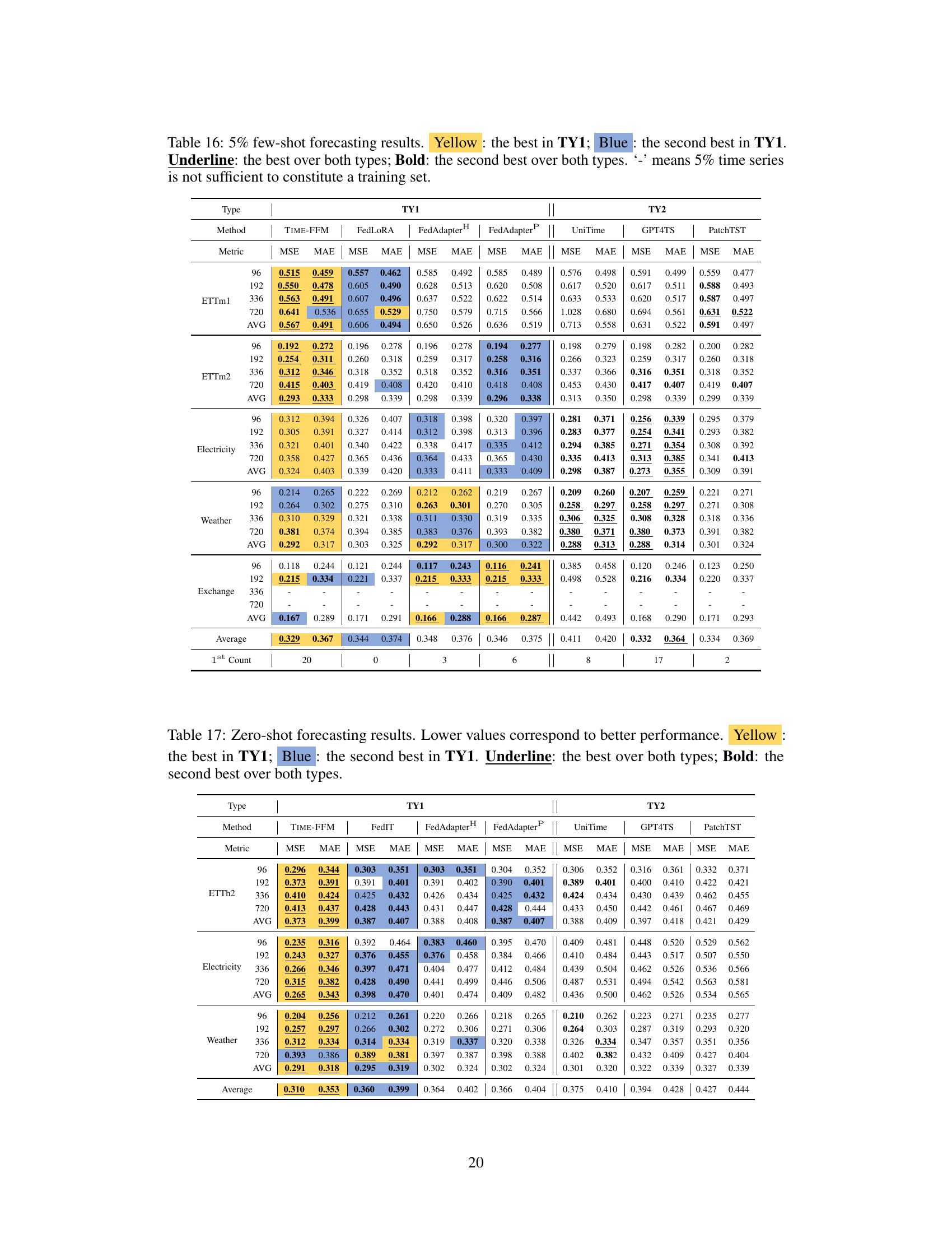
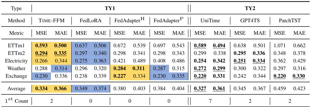
This table presents the results of a 5% few-shot forecasting experiment. It compares the performance of different models (TIME-FFM and several baselines) across various time series datasets, in a setting where only 5% of the data is used for training. The table highlights the best performing model within two categories (TY1 and TY2) and overall, using color-coding to differentiate the top performers.

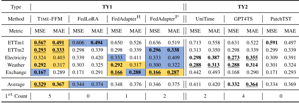
This table presents the results of zero-shot forecasting experiments. The models were trained on ETTh1, ETTm1, and ETTm2 and then tested on ETTh2, Electricity, and Weather datasets without further fine-tuning. The table compares the performance of TIME-FFM against other federated learning (TY1) and centralized (TY2) methods using MSE and MAE metrics. Color-coding highlights the best and second-best results within each category, and underlines highlight the overall best performers.

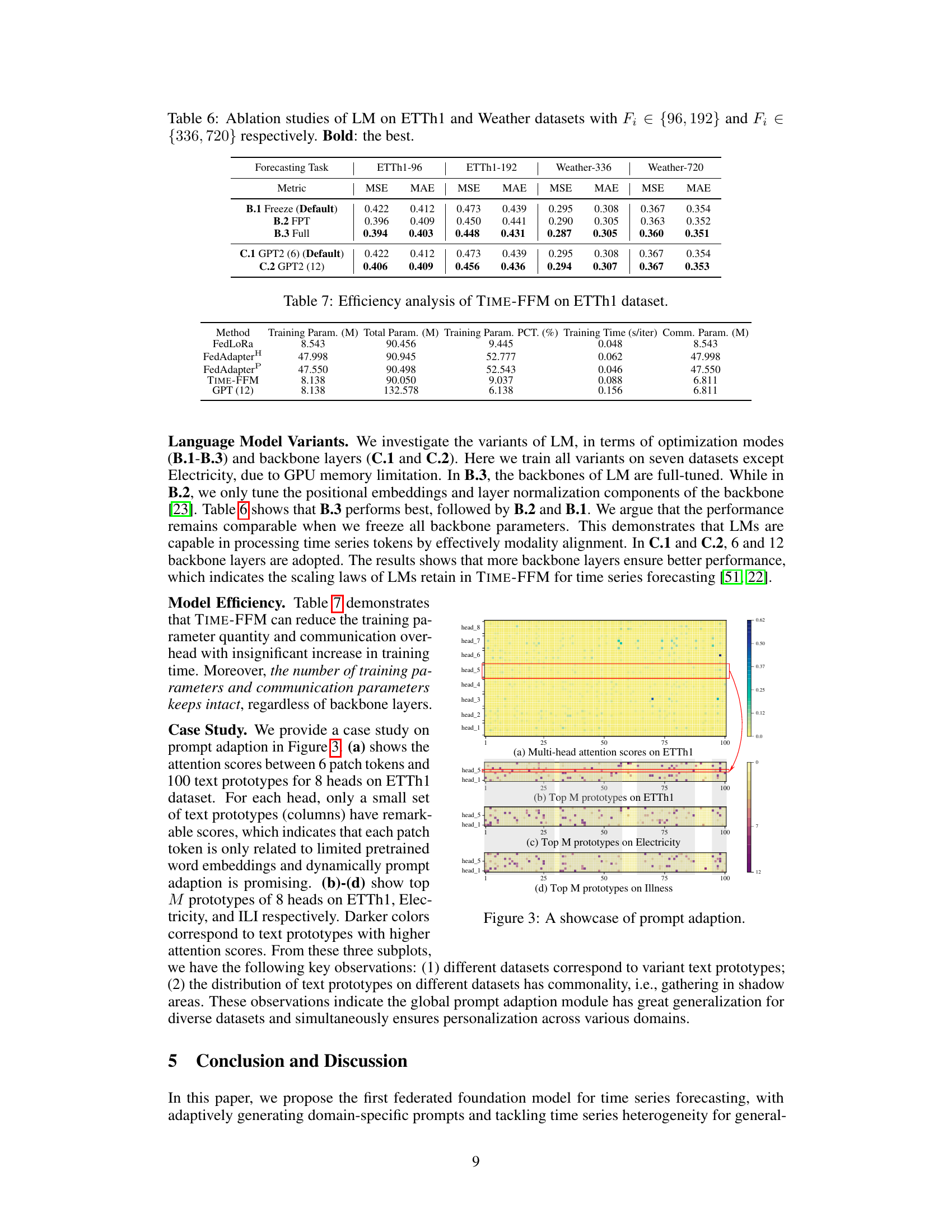
This table presents the ablation study results for the proposed TIME-FFM model. It shows the impact of different components of the model on forecasting performance using ETTh1 and ILI datasets with two different prediction window sizes. The variations studied include removing the prompt adaption module, using explicit instructions instead of adaptive prompts, removing the personalized prediction heads, removing all the proposed components, and using a distributed version of TIME-FFM without global model aggregation. The results are presented as Mean Squared Error (MSE) and Mean Absolute Error (MAE) metrics.

This ablation study investigates the impact of using different Language Model (LM) variants on the forecasting performance. Three different LM optimization modes were tested: freezing all parameters, fine-tuning positional embeddings and layer normalization, and full fine-tuning. Additionally, two different GPT2 backbone sizes (6 and 12 layers) were evaluated. The results demonstrate the impact of each approach on Mean Squared Error (MSE) and Mean Absolute Error (MAE) across different forecasting horizons (F₁).

This table presents the efficiency analysis of the proposed TIME-FFM model and other baseline models (FedLoRA, FedAdapterH, FedAdapterP, and GPT(12)) on the ETTh1 dataset. The metrics presented include training parameters (in millions), total parameters (in millions), training parameter percentage, training time per iteration (in seconds), and communication parameters (in millions). This table demonstrates the efficiency of the TIME-FFM model compared to other methods in terms of the number of parameters used and training time.

This table provides detailed information about the eight benchmark datasets used in the paper’s experiments. For each dataset, it lists the number of channels (ci), the dataset size (number of samples in training, validation, and test sets), the batch size used during training, the oversampling times (relevant to data augmentation), the frequency of the time series data (e.g., 1 hour, 15 minutes), and the application domain from which the data originates. This information is crucial for understanding the experimental setup and the generalizability of the results.

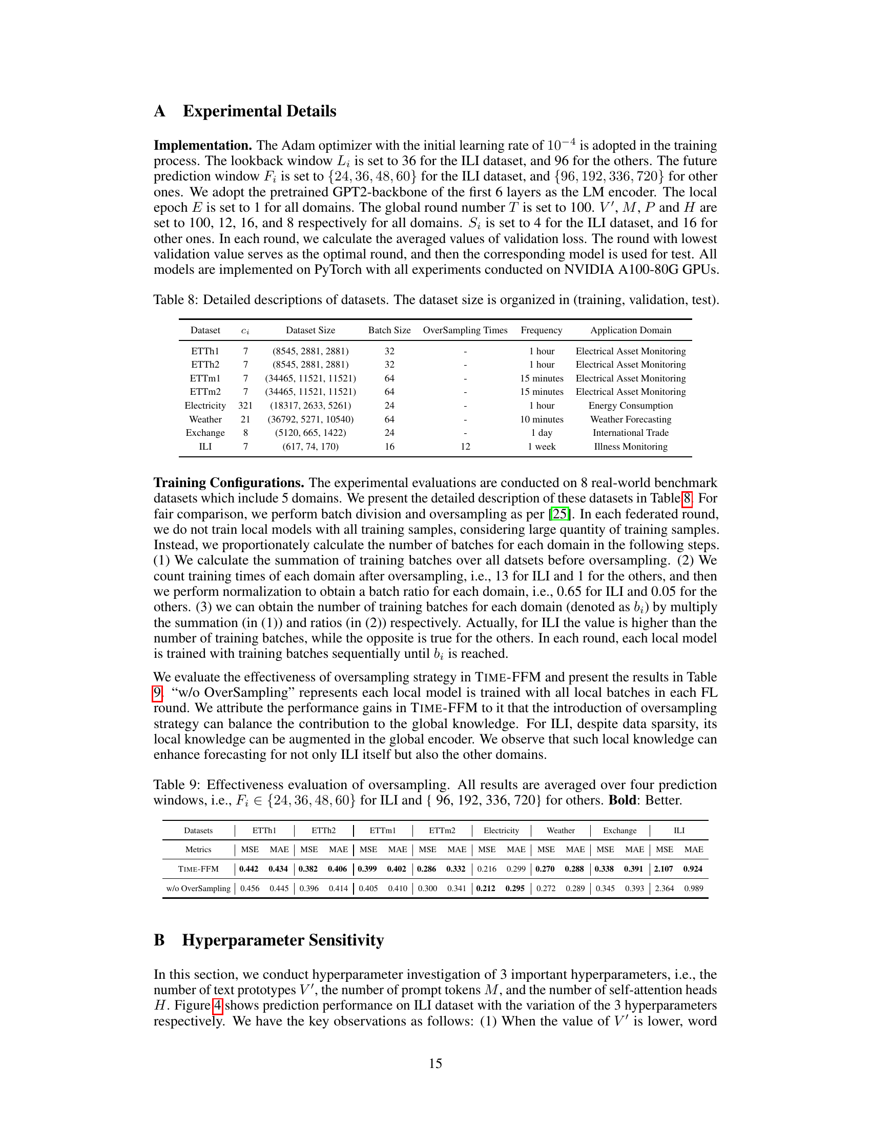
This table presents the results of an experiment to evaluate the effectiveness of oversampling in the TIME-FFM model. It compares the model’s performance with and without oversampling across eight benchmark datasets from various domains. The metrics used for evaluation are Mean Squared Error (MSE) and Mean Absolute Error (MAE). The bold values indicate better performance compared to the no oversampling strategy.

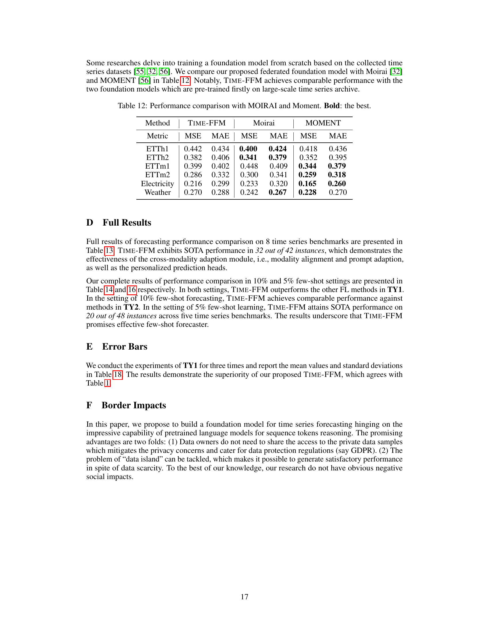
This table compares the performance of TIME-FFM against two other federated learning methods, PatchTST-FL and DLinear-FL, across eight benchmark datasets representing various domains. The metrics used are MSE (Mean Squared Error) and MAE (Mean Absolute Error). The results highlight the superior performance of TIME-FFM in terms of both MSE and MAE on average across the datasets, indicating its effectiveness and robustness compared to the other federated learning methods.

This table compares the forecasting performance of TIME-FFM with three other state-of-the-art time series forecasting models: iTransformer, N-BEATS, and Crossformer. The metrics used are Mean Squared Error (MSE) and Mean Absolute Error (MAE). The results are averaged across multiple datasets (ETTm2, Weather, and Exchange). The bold values indicate the best performance achieved by any method for each metric and dataset.

This table compares the performance of TIME-FFM against two other foundation models, Moirai and MOMENT, across six benchmark datasets. The metrics used are MSE and MAE, representing Mean Squared Error and Mean Absolute Error respectively, which are common metrics for evaluating the accuracy of time series forecasting models. Lower values indicate better performance. The table highlights the competitive performance of TIME-FFM, particularly showing better performance in several instances. This comparison aims to illustrate TIME-FFM’s performance against existing foundation models trained from scratch on large-scale time series data.

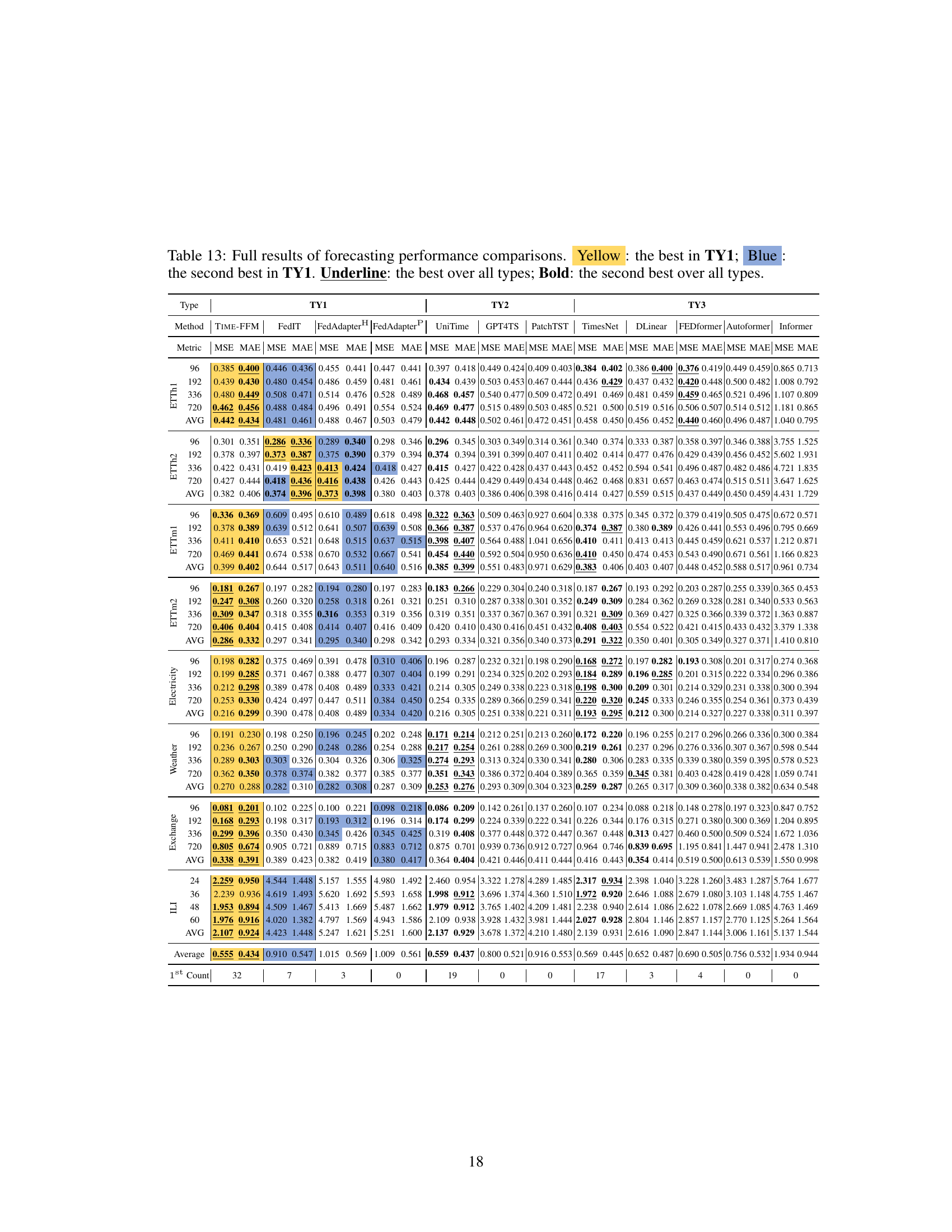
This table presents a comparison of forecasting performance across various methods categorized into three types (TY1, TY2, and TY3). It shows Mean Squared Error (MSE) and Mean Absolute Error (MAE) for eight different datasets and four prediction window lengths (F1). The best and second-best performing methods within TY1, and overall best and second-best methods across all three types are highlighted.

This table presents a comparison of forecasting performance across various methods categorized into three types: federated fine-tuning methods (TY1), across-dataset centralized methods (TY2), and dataset-specific centralized methods (TY3). The metrics used are Mean Squared Error (MSE) and Mean Absolute Error (MAE), averaged over four different prediction window lengths. The table highlights the best (yellow) and second-best (blue) performing methods within each category (TY1) and overall (underlined and bolded). Complete results can be found in Table 13.

This table presents a comparison of the forecasting performance of TIME-FFM against various baseline methods across eight benchmark datasets. The metrics used are Mean Squared Error (MSE) and Mean Absolute Error (MAE), averaged over four different prediction window lengths. The table highlights the best (yellow) and second best (blue) performers within the three method categories (TY1, TY2, and TY3), as well as the overall best and second best performers across all categories. Full results are provided in a separate table (Table 13).
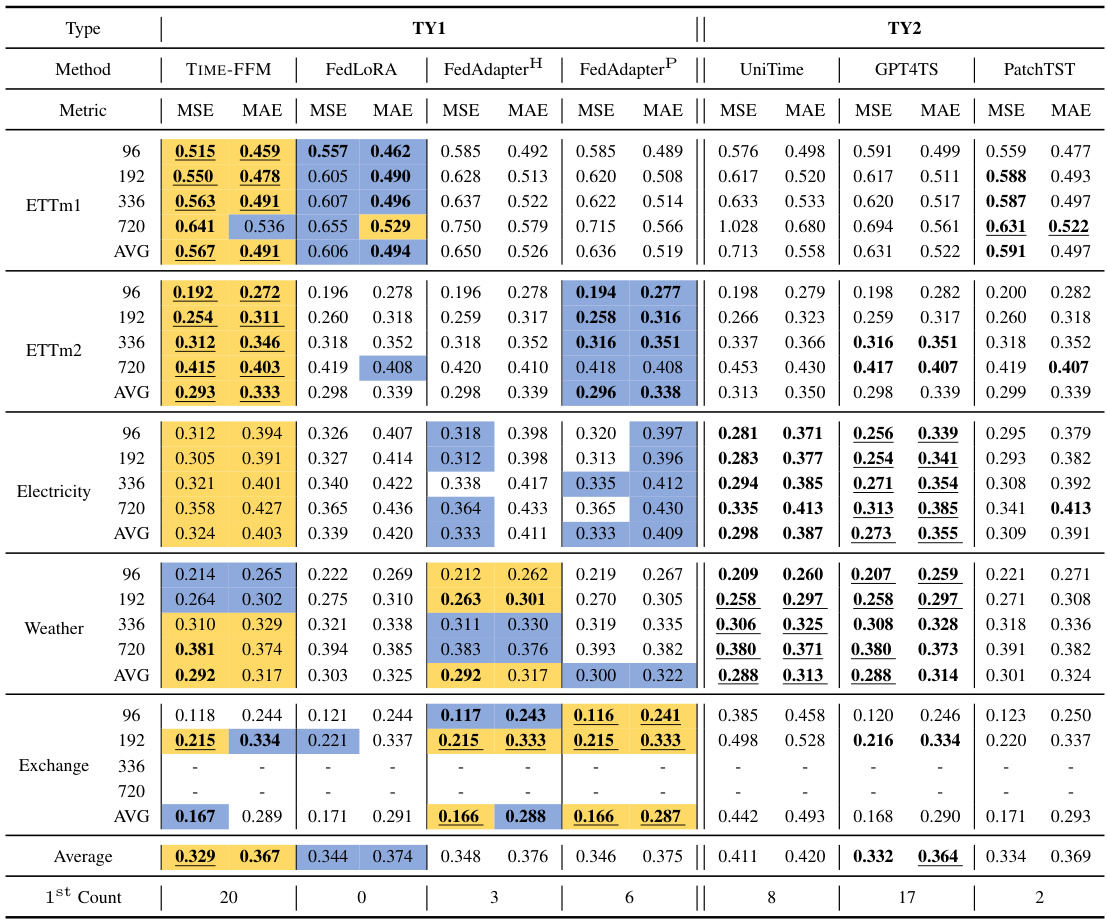
This table compares the forecasting performance of TIME-FFM against several baseline methods across eight benchmark datasets. The metrics used are MSE and MAE, averaged over four prediction windows. The table highlights the best and second-best performing models within each category (TY1, TY2, TY3), overall best, and overall second-best. Color-coding indicates performance within the TY1 category. Full results can be found in Table 13.

This table presents a comparison of the forecasting performance of TIME-FFM against various baseline methods across eight benchmark datasets. The metrics used are MSE and MAE, averaged across four prediction window lengths for each dataset. The table highlights the best performing methods within three categories: federated fine-tuning methods (TY1), centralized cross-dataset methods (TY2), and dataset-specific centralized methods (TY3). Color-coding indicates the best and second-best performance within TY1 and overall.

This table presents the mean and standard deviation of the MSE and MAE metrics across three runs for each of the eight datasets in TY1 (federated fine-tuning methods). It provides a quantitative measure of the stability and reliability of the results obtained by different federated learning methods. Lower values generally indicate better performance.
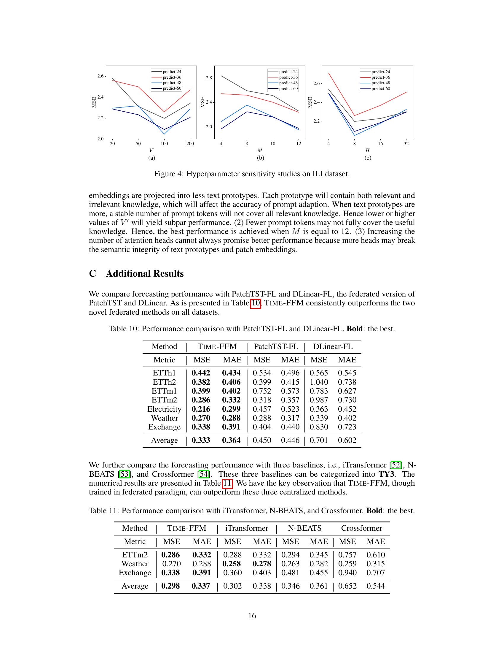
Full paper#
