↗ OpenReview ↗ NeurIPS Homepage ↗ Chat
TL;DR#
Current machine learning struggles to formally integrate prior knowledge into predictive models, limiting nuanced analysis and accessibility for non-specialists. This often restricts the use of probabilistic models to specialists due to the expertise needed for proper integration. This paper aims to overcome these limitations.
This research introduces LLM Processes, a regression model that leverages Large Language Models (LLMs) to process numerical data and generate probabilistic predictions, guided by user-provided natural language descriptions. The work demonstrates effective prompting techniques for eliciting coherent predictive distributions from LLMs, showcasing enhanced regression performance. Moreover, the study highlights how text significantly boosts predictive accuracy and reflects qualitative aspects quantitatively, paving the way for more advanced, context-aware AI systems.
Key Takeaways#
Why does it matter?#
This paper is crucial for researchers seeking to integrate prior knowledge into predictive models, particularly those using large language models. It offers practical methods for eliciting numerical predictive distributions from LLMs, improves predictive performance, and opens avenues for incorporating qualitative descriptions into quantitative predictions. This will drive the development of more nuanced and context-aware AI systems.
Visual Insights#
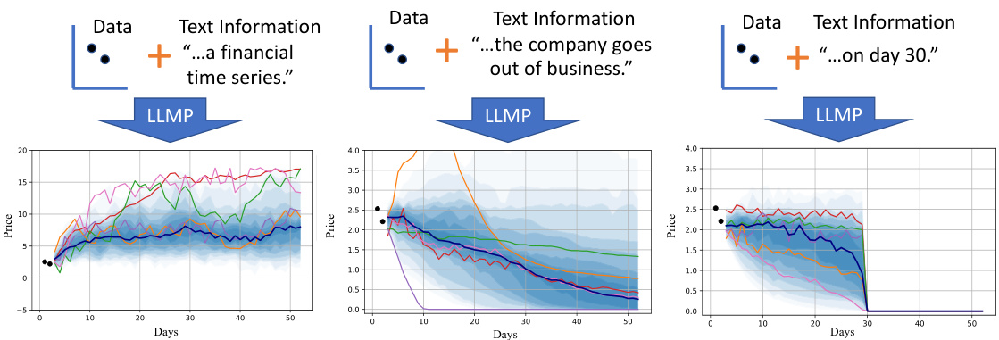
This figure shows three examples of predictive distributions generated by an LLMP (Large Language Model Process). Each example demonstrates how the model incorporates both numerical data (shown as points) and textual information to produce a predictive distribution. The text influences the shape and range of the prediction. The faded blue shows the 10th percentile of 50 samples from the model, the darker blue line is the median and several individual sample lines are shown in various colors. The examples show how different text descriptions can lead to different predictions.

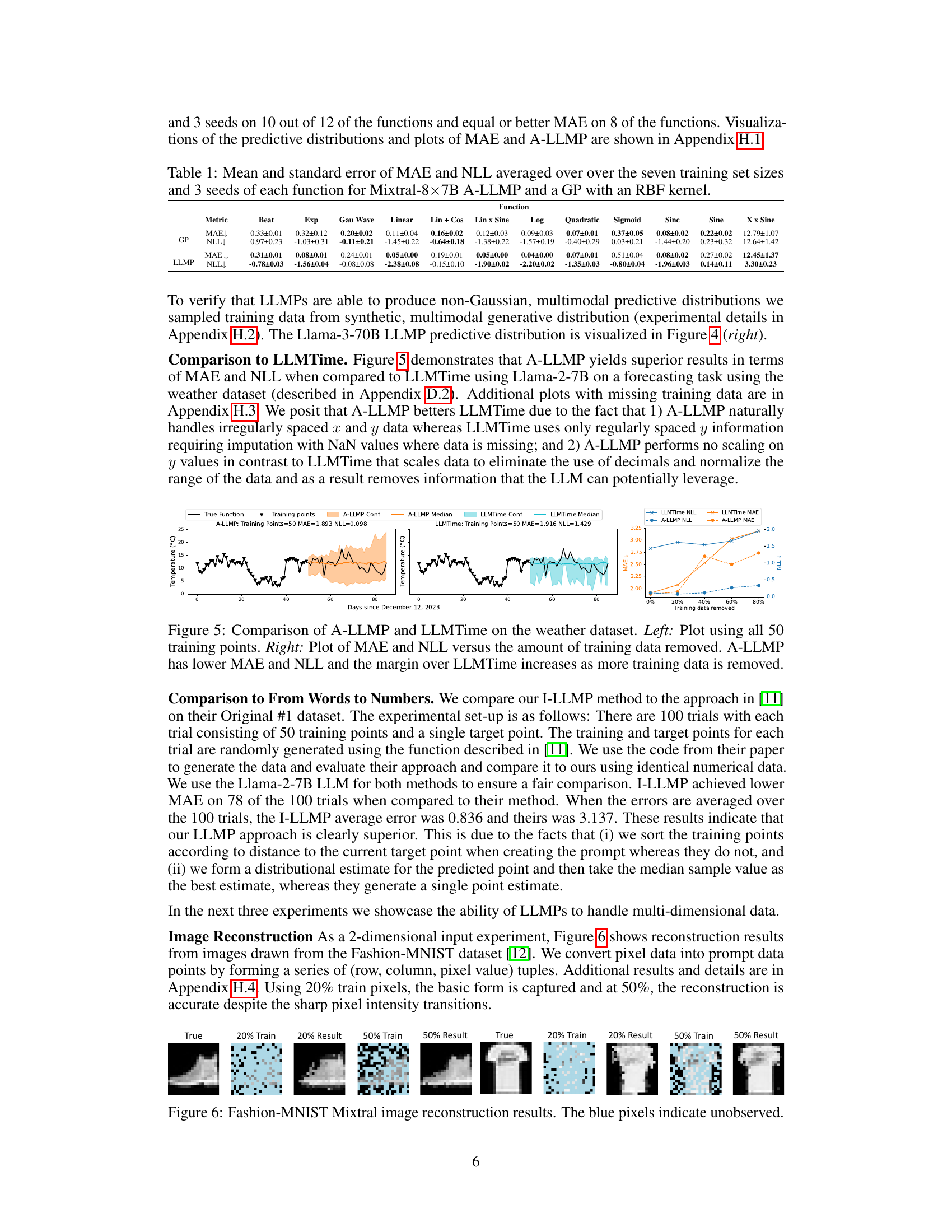
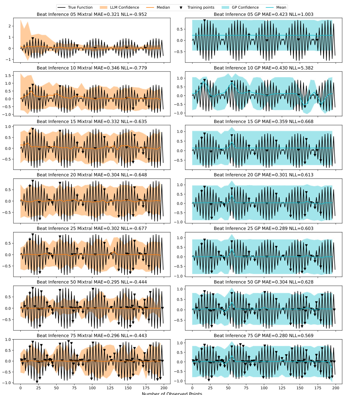
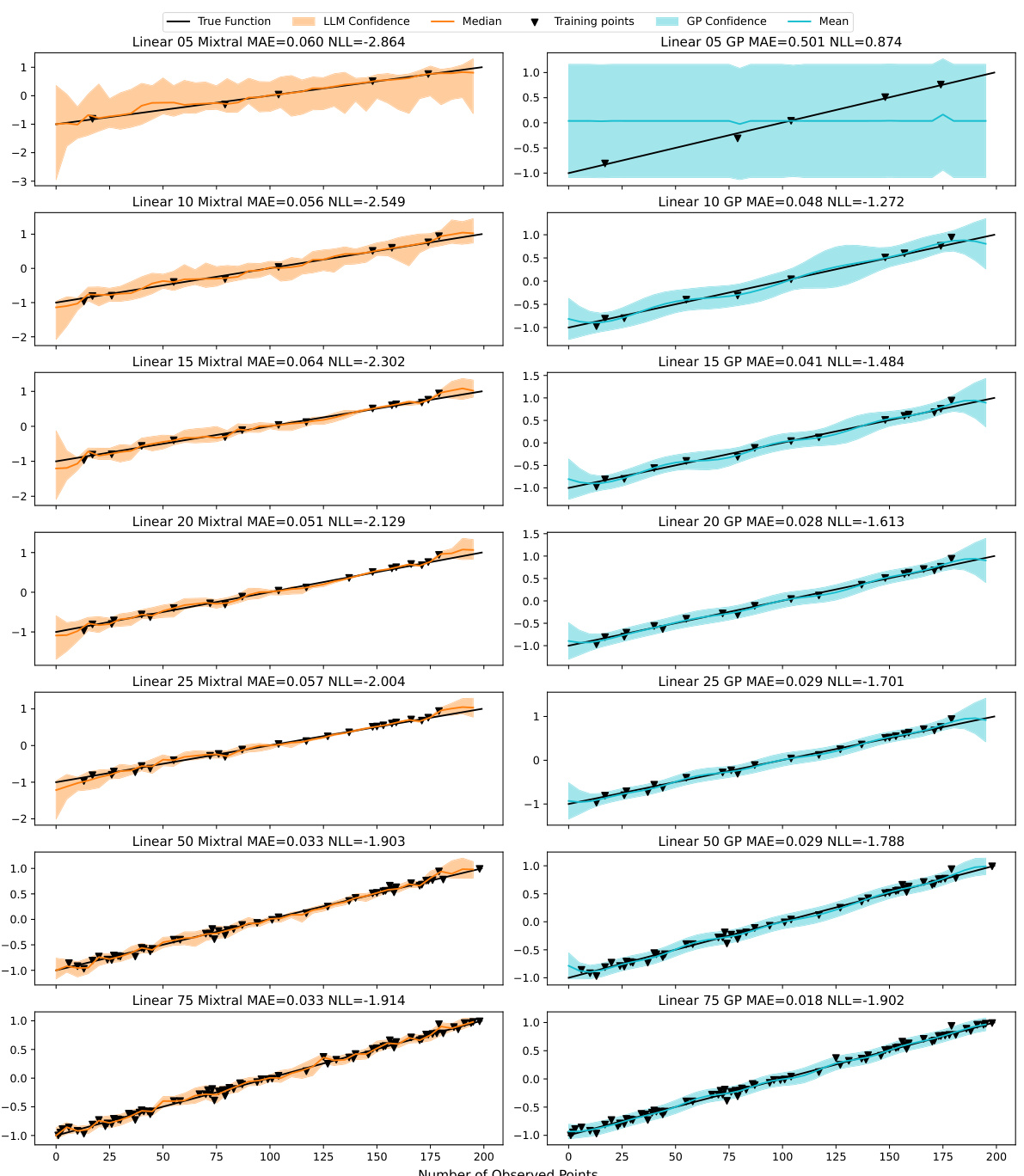
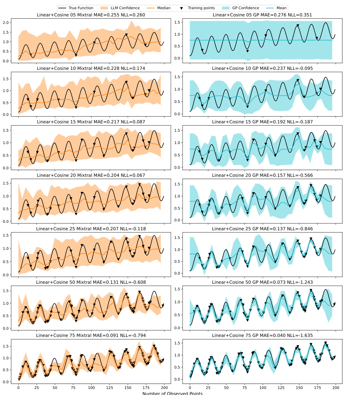
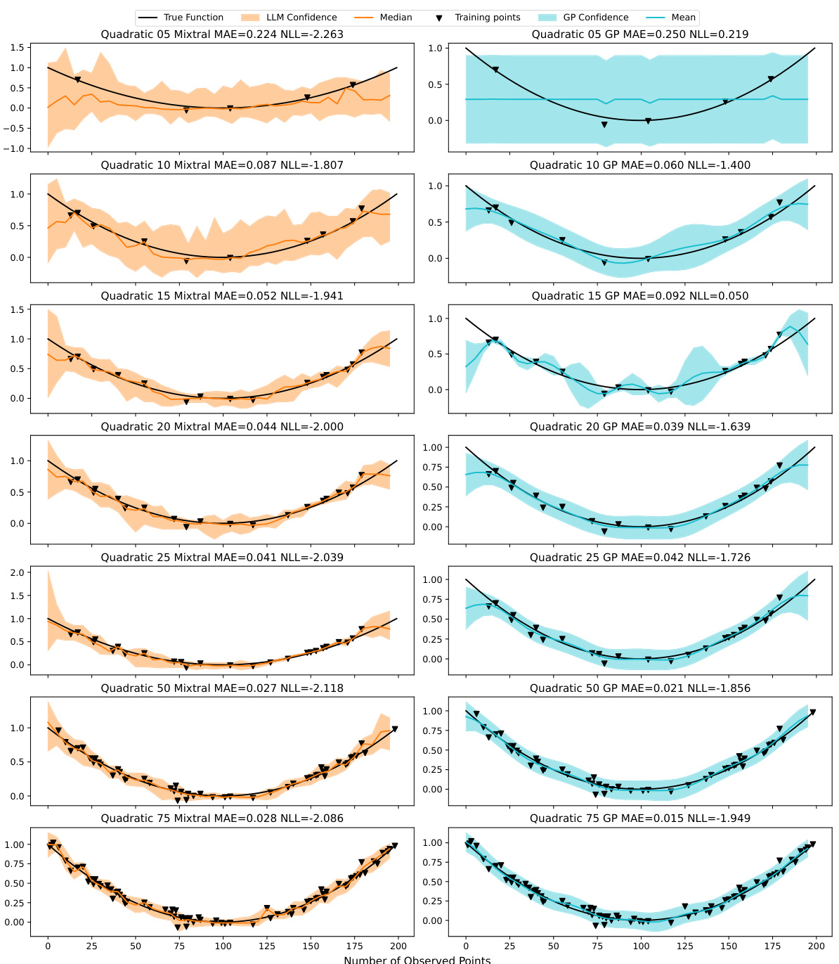
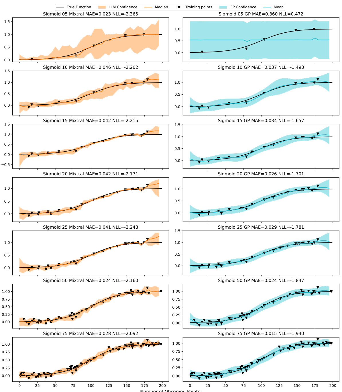
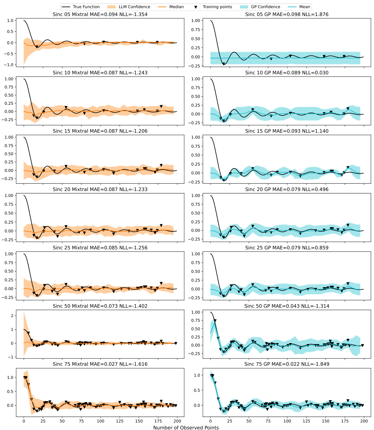
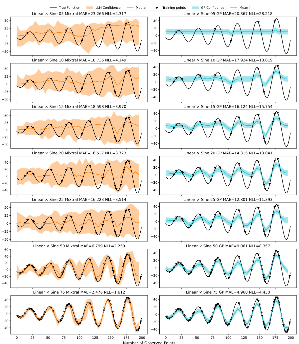
This table presents a comparison of the Mean Absolute Error (MAE) and Negative Log-Likelihood (NLL) achieved by the Mixtral-8×7B A-LLMP model and a Gaussian Process (GP) model with a radial basis function (RBF) kernel. The comparison is made across seven different training set sizes (5, 10, 15, 20, 25, 50, and 75 data points) and three random seeds for each of twelve different synthetic functions. The results show the average MAE and NLL for each model, along with the standard error, providing insights into the relative performance of each model under varying data conditions.
In-depth insights#
LLM Numerical Regression#
LLM Numerical Regression explores leveraging Large Language Models (LLMs) for numerical regression tasks. This approach presents a unique paradigm shift, moving beyond traditional machine learning methods by utilizing the inherent knowledge and pattern-recognition capabilities of LLMs. A key aspect is the ability to seamlessly integrate prior knowledge and contextual information through natural language prompts, enabling more nuanced and context-aware analyses. This contrasts with traditional methods that often require complex mathematical formulations of prior beliefs. The effectiveness of LLM Numerical Regression hinges on carefully designed prompting strategies. Prompt engineering plays a crucial role in eliciting coherent and reliable numerical predictive distributions from the LLM, which are then used for the regression. The method’s success is demonstrated by its competitive performance against established methods like Gaussian Processes on various benchmark datasets. However, challenges remain, such as managing the inherent stochasticity of LLMs and addressing issues like computational cost and potential biases encoded within the pretrained models. This new field offers promising avenues for enhancing both predictive accuracy and interpretability in regression.
Prompt Engineering for LLMs#
Prompt engineering for LLMs is crucial for effective results, as the quality and structure of prompts significantly impact the model’s output. Careful consideration of prompt design can elicit more accurate, coherent, and nuanced responses. This includes experimenting with different prompt formats and structures, such as the use of clear instructions, few-shot examples, and chain-of-thought prompting to guide the model’s reasoning process. Furthermore, prompt engineering is an iterative process, involving experimentation and refinement based on observed outputs. Analyzing the model’s responses helps identify areas where the prompt can be improved. The contextual information provided within a prompt should be relevant and appropriately weighted, while also considering the need to manage prompt length limitations of large language models. Understanding the LLM’s biases and limitations is essential when engineering prompts, recognizing that the model’s output is affected by its training data and inherent limitations. Measuring prompt effectiveness relies on clearly defined metrics and statistical significance testing.
Autoregressive LLMs#
Autoregressive Language Models (LLMs) are a class of LLMs that predict the probability of the next token in a sequence, conditioned on all preceding tokens. This approach is particularly useful for text generation because it allows the model to produce coherent and contextually relevant text. A key advantage of autoregressive LLMs is their ability to generate long, complex sequences of text, which is a significant challenge for other types of LLMs. However, they also present some challenges. For example, autoregressive LLMs can be computationally expensive, and they can be difficult to train and tune. Furthermore, because they generate text sequentially, they are prone to errors and inconsistencies if the model makes an early prediction mistake. The sequential nature of autoregressive LLMs means that predictions made later in the sequence are conditioned on earlier ones, potentially amplifying initial errors. Efficient sampling methods such as top-p or nucleus sampling are often employed to mitigate this issue. In summary, autoregressive LLMs are powerful and versatile tools for various natural language processing tasks, especially text generation, but careful consideration should be given to the computational cost, potential for error propagation, and the need for efficient sampling methods.
Incorporating Textual Info#
Incorporating textual information into numerical prediction models presents a significant challenge, but offers the potential for enhanced accuracy and context-awareness. The integration of textual data allows for the inclusion of expert knowledge, qualitative descriptions, and problem-specific details that are often difficult to represent numerically. This is particularly useful when dealing with messy or incomplete datasets, or where prior knowledge about the problem domain is available. One of the main strategies is to leverage the rich hypothesis space implicitly encoded in Large Language Models (LLMs). By effectively prompting LLMs, the goal is to elicit coherent numerical predictive distributions that reflect the information provided in the text. However, this process presents considerable challenges, such as ensuring consistency, handling inconsistencies in the LLM’s responses, and effectively managing the computational cost of eliciting these distributions. The effectiveness of this approach relies heavily on the quality of prompting techniques, the ability of the LLM to capture and translate qualitative descriptions into quantitative measures, and the selection of an appropriate statistical framework for handling uncertainty.
LLMP Limitations#
LLM Processes, while innovative, face limitations stemming from their reliance on Large Language Models (LLMs). LLMPs inherit the limitations of LLMs, such as context window limitations restricting the size of problems they can handle and the amount of textual information they can process. The computational cost of LLMPs is significantly higher than standard regression methods. Interpretability is another major limitation: unlike Gaussian Processes, LLMPs lack explicit prior encoding, necessitating empirical demonstration of well-calibrated predictions. Additionally, the impact of LLM biases on LLMP output is unclear and requires further research. There’s also the challenge of evaluating the full societal impact of LLMPs; while they offer great potential in numerous fields, the possibility of misuse and unintended consequences needs careful consideration. Furthermore, the ability of LLMPs to generalize to unseen data and their sensitivity to prompt engineering needs more thorough investigation. Ultimately, further research is crucial to address these limitations and enhance the trustworthiness and applicability of LLMPs.
More visual insights#
More on figures

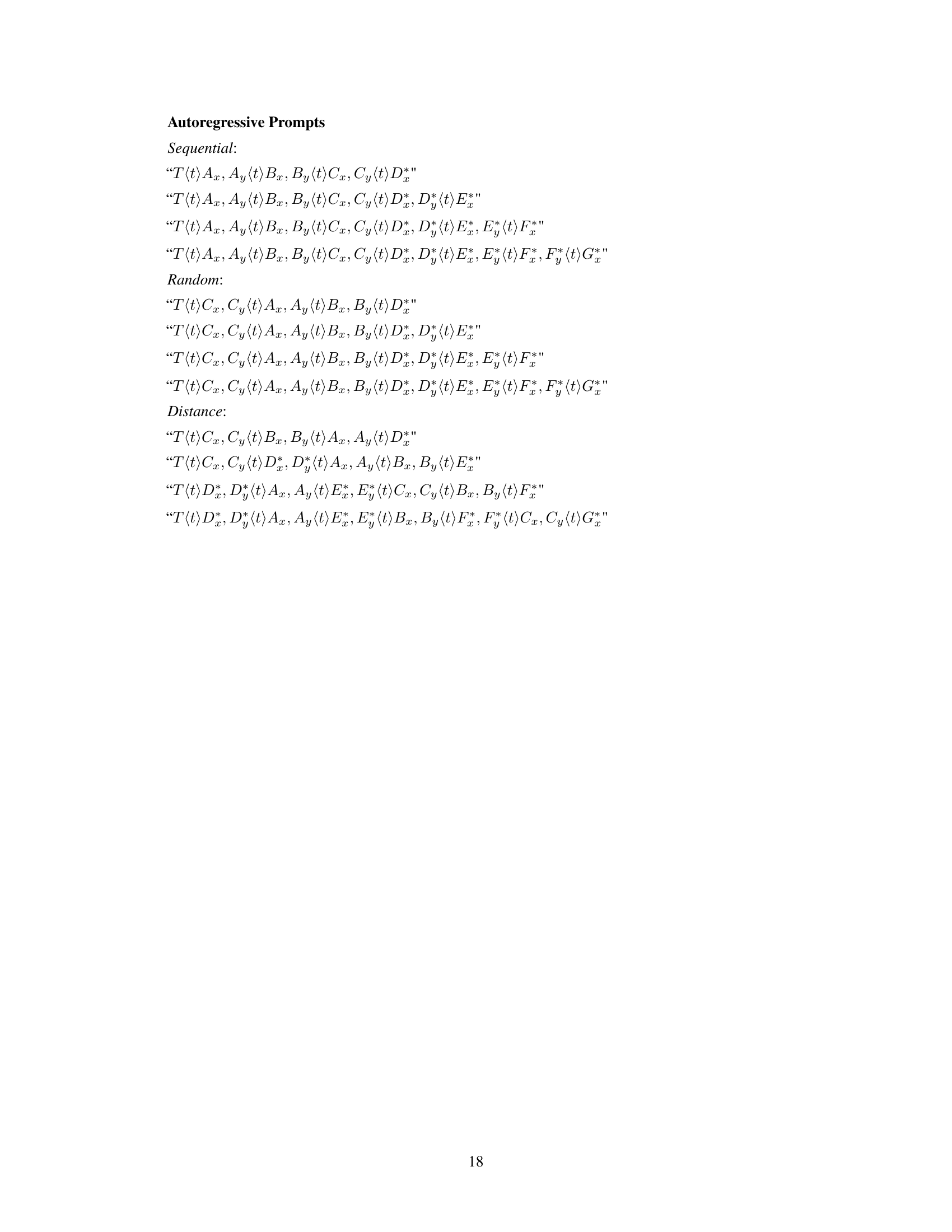
This figure illustrates two different sampling methods from a large language model (LLM) for generating numerical predictions. The independent marginal approach samples from the LLM’s predictive distribution for each target location independently. The autoregressive method, in contrast, conditions the LLM’s prediction on the previously generated values for other target points, creating a richer joint predictive distribution that captures dependencies between variables. Both methods show how the LLM generates multiple samples (‘N samples’) at each target point, allowing for the estimation of uncertainty in the predictions. The median of these samples represents the most likely prediction.

The figure shows three examples of predictive distributions generated by an LLM Process (LLMP). Each example demonstrates how the LLMP combines numerical data with textual descriptions to produce a predictive distribution. The faded blue area represents the 10th to 90th percentile range of 50 samples, the dark blue line represents the median, and the other colored lines show five randomly selected individual samples from the predictive distribution. The x-axis represents time (days), and the y-axis represents the price. Each example highlights the impact of incorporating textual information (different sentences describing the underlying process) into the prediction.

This figure displays three examples of predictive distributions generated by an LLMP (Large Language Model Process). Each example shows how the model incorporates both numerical data (a time series of prices) and textual information (describing the context of the data) to create a probability distribution of future price predictions. The faded blue represents the 10th percentile of 50 samples, the dark blue line is the median, and additional lines in various colours show other randomly selected samples from the model’s prediction. The textual information significantly influences the predicted price distribution in each case.

This figure displays three examples of predictive distributions generated by an LLMP (Large Language Model Process). Each example shows how the model incorporates both numerical data (a time series) and textual information to produce a predictive distribution. The shaded blue area represents the 10th to 90th percentiles of 50 samples, the dark blue line represents the median prediction, and the colored lines represent five randomly selected samples. The text information conditions the model’s prediction, demonstrating how prior knowledge can shape the output.

This figure shows three examples of predictive distributions generated by an LLMP (Large Language Model Process). Each example uses different text information in addition to numerical data. The faded blue shows the 10th percentile, the dark blue shows the median, and the other colours represent five random samples from the 50 generated. This illustrates how LLMPs can incorporate textual information into their probabilistic predictions.

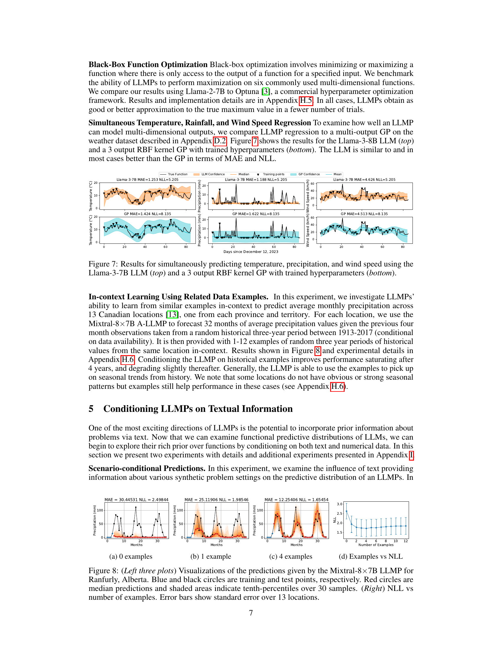
The figure shows the results of simultaneously predicting temperature, precipitation, and wind speed using Llama-3-7B LLM and comparing it to a Gaussian Process (GP) with 3 outputs. The top row presents the results of the LLM, showing the true values, LLM confidence intervals, median predictions, and training points. The bottom row presents the results of the GP, similarly displaying the true values, GP confidence intervals, mean predictions, and training points. The figure demonstrates the ability of LLMs to effectively model multi-dimensional outputs, highlighting their potential for complex prediction tasks.

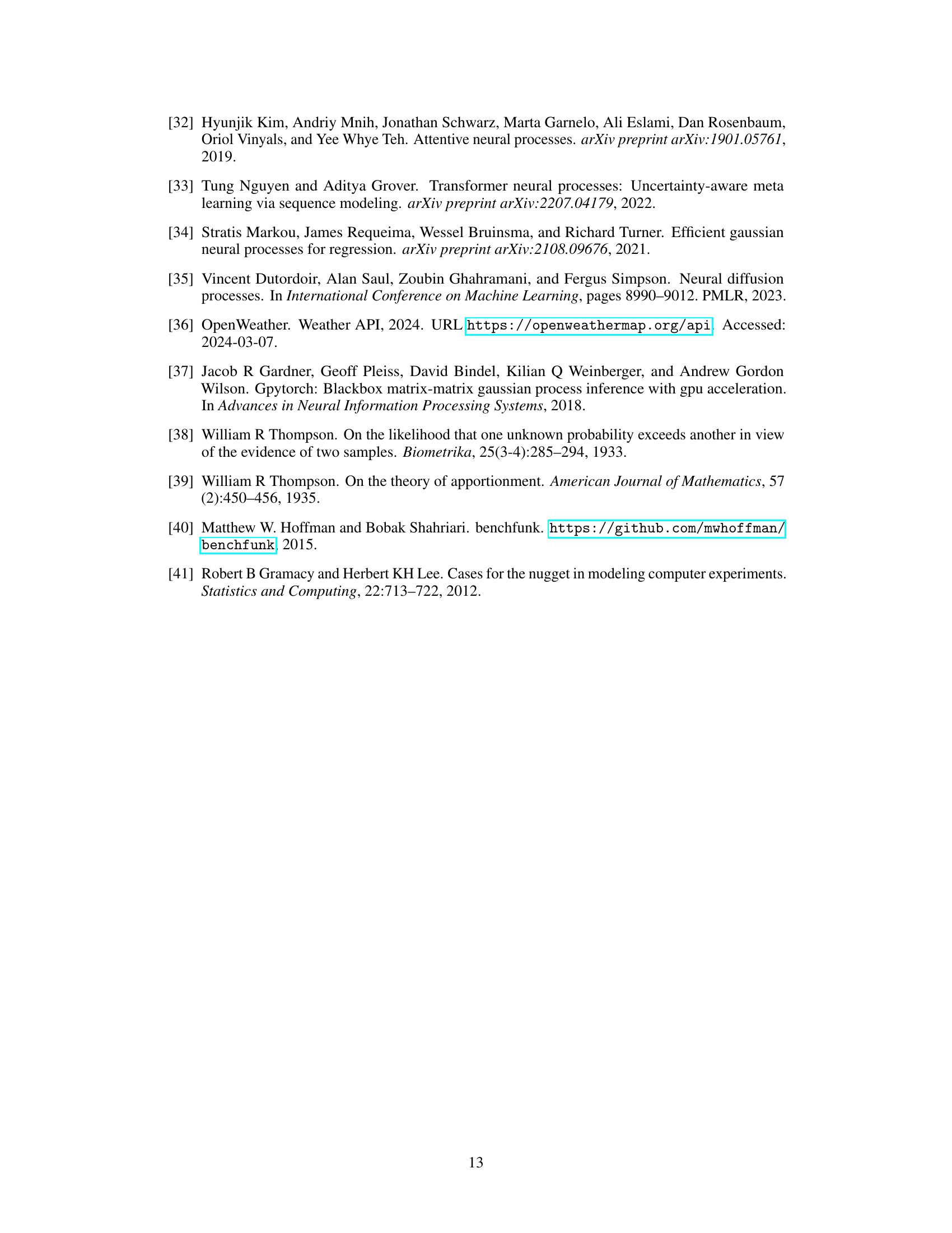
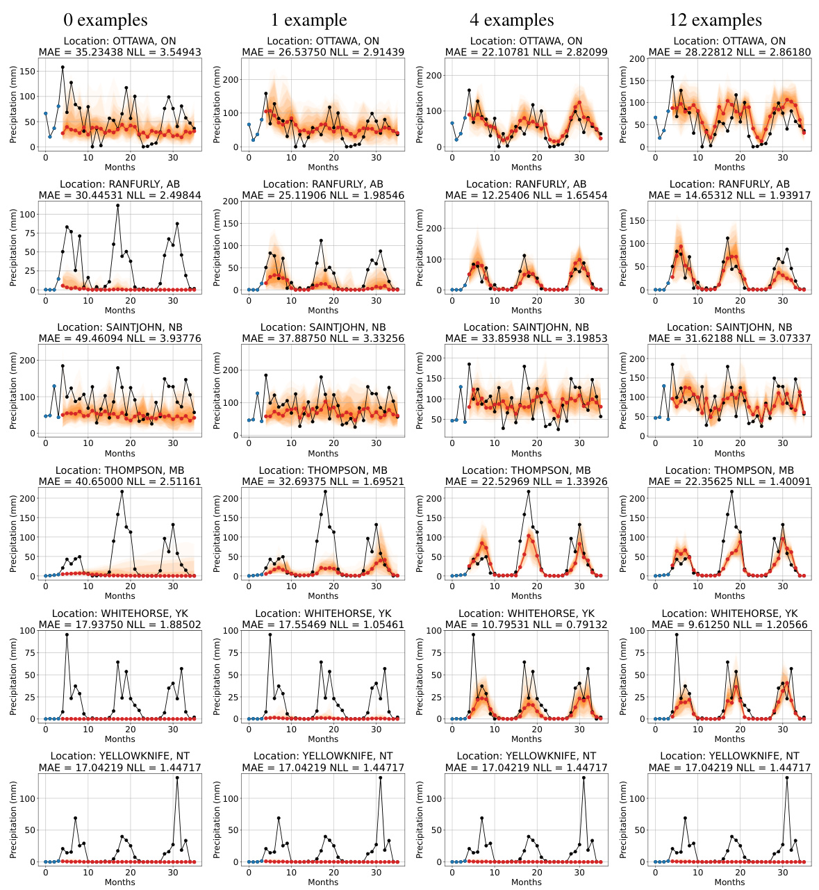
This figure displays the results of an experiment investigating in-context learning using the Mixtral-8x7B LLMP to predict average monthly precipitation in Ranfurly, Alberta. The left three plots show visualizations of predictive distributions for various numbers of examples. Each plot shows 32 months of precipitation forecasts (red) compared to actual data (blue), illustrating how model performance improves as the number of in-context examples increases. The right plot summarizes the average negative log-likelihood (NLL) across 13 locations, showing a clear improvement in prediction accuracy with more examples. Error bars indicate standard error.
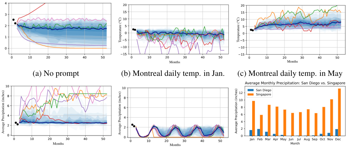
This figure shows three examples of predictive distributions generated by an LLMP (Large Language Model Process). Each example demonstrates how the model incorporates both numerical data (shown as a time series) and text information to generate a predictive distribution. The text information provides context and influences the shape of the distribution. The faded blue represents the 10th percentile, the dark blue line represents the median, and the other lines show five randomly selected samples from the 50 samples used to generate the predictive distribution.

This figure shows three examples of predictive distributions generated by an LLM Process (LLMP). Each example demonstrates how an LLMP can incorporate both numerical data (a time series) and textual information to produce a predictive distribution. The faded blue represents the 10th percentiles, the dark blue line is the median prediction, and the various coloured lines show five random samples from the predictive distribution. The text information conditions the model on different assumptions about the data generating process, resulting in different shapes and locations of the predicted distributions.
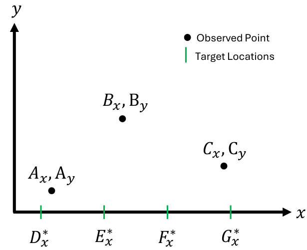
This figure illustrates the two different sampling methods used to obtain predictive distributions from an LLM: independent marginal sampling and autoregressive sampling. In independent marginal sampling, the LLM is prompted separately for each target location, providing marginal distributions. In autoregressive sampling, the LLM receives the previous predictions as part of the prompt, enabling it to model dependencies between output variables and producing a richer, potentially more accurate, joint distribution.
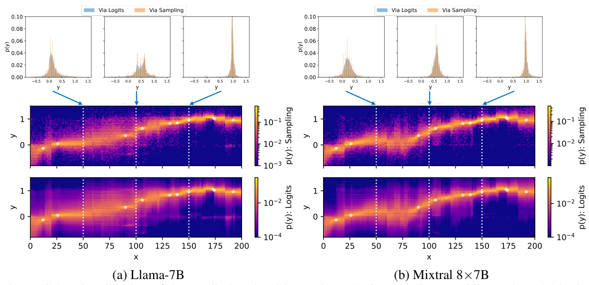
This figure displays three examples of predictive distributions generated by an LLM Process (LLMP). Each example shows how the LLMP incorporates both numerical data (a time series) and textual information to generate a predictive distribution. The faded blue represents the 10th percentile of 50 samples, the dark blue line is the median, and the different colored lines show five randomly selected samples. The textual information provided to the model influences the shape of the predictive distribution, demonstrating the ability of LLMPs to incorporate qualitative descriptions into quantitative predictions.
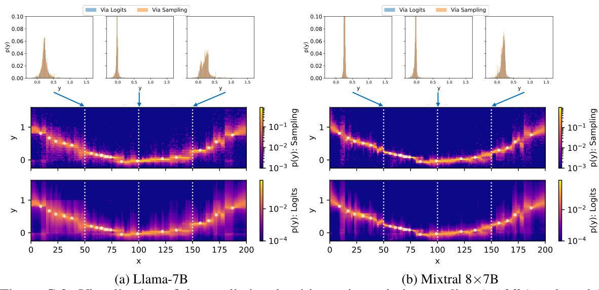
This figure demonstrates the ability of the LLM Process (LLMP) model to generate predictive distributions conditioned on both numerical data and text information. Three examples are shown illustrating different scenarios. Each panel shows a predictive distribution (faded blue shows the 10th percentiles from 50 samples, dark blue shows the median and other lines show five random samples) for the price over time, with different text prompts giving additional context for each scenario. The plots demonstrate that the LLMP can incorporate text to generate context-aware predictions.

This figure displays three examples of predictive distributions generated by an LLMP (Large Language Model Process). Each example shows how the model incorporates both numerical data (in the form of a time series) and textual information to generate a predictive distribution. The faded blue represents the 10th percentiles of 50 samples, the dark blue line shows the median, and the different coloured lines represent five individual samples. The examples highlight how textual descriptions influence the shape and range of the predictive distribution, demonstrating the model’s ability to incorporate prior knowledge or contextual information into its predictions.

This figure visualizes predictive distributions generated by an LLM Process (LLMP), a model that incorporates both data and textual information. Three examples are shown, each illustrating how the LLMP produces predictive distributions based on different datasets and textual descriptions. The plots show the tenth percentiles from 50 samples (faded blue), the median (dark blue), and five individual samples (various colours). The figure highlights the model’s ability to integrate qualitative information (text) and quantitative data for improved probabilistic predictions.

The figure displays three examples of predictive distributions generated by an LLMP (Large Language Model Process). Each example shows how the model incorporates both numerical data (a time series) and textual information to produce a probability distribution over future values. The shaded blue areas represent the 10th to 90th percentiles from 50 samples generated by the LLMP, giving a sense of the model’s uncertainty. The darker blue line is the median prediction, and individual sample predictions are shown in different colors. The text descriptions condition the model on different scenarios or prior knowledge. This illustrates the model’s ability to integrate both numerical data and textual information for prediction and to express uncertainty in its predictions.

This figure shows three examples of predictive distributions generated by an LLMP (Large Language Model Process). Each example includes a time series dataset and a text description. The text description provides additional context about the data, such as whether it is a financial time series or the company’s financial status. The tenth percentiles from 50 samples are shown in light blue, the median is shown in dark blue, and five random samples are shown in various colours. This demonstrates the ability of the LLMP to incorporate textual information into its numerical predictions, producing predictive distributions that reflect qualitative descriptions.

This figure shows three examples of predictive distributions generated by an LLMP (LLM Process). Each example uses a different text description to condition the model, demonstrating how the text influences the resulting distribution. The dark blue line is the median prediction, while the lighter blue represents the 10th percentile range, showing uncertainty. Individual sample predictions are shown in different colors. The plots illustrate how LLMPs combine numerical data and natural language to make probabilistic predictions, showcasing context-aware analyses.

This figure displays three examples of predictive distributions generated by an LLMP (Large Language Model Process). Each example shows how the model incorporates both numerical data (shown as a time series) and textual information (a short description of the data’s context) to produce a probabilistic prediction. The faded blue area represents the range containing the 10th to 90th percentiles of 50 predictions, the dark blue line shows the median prediction, and the other colored lines highlight five individual sample predictions. This illustrates the LLMP’s ability to integrate textual context into numerical predictions, thus providing a more nuanced and informative forecast.

This figure shows three examples of predictive distributions generated by an LLMP (Large Language Model Process). Each example uses different text information to guide the model in addition to numerical data. The faded blue represents the 10th percentile, dark blue represents the median, and individual colored lines depict five random samples from 50 generated samples. The purpose is to illustrate how adding textual information influences the shape and uncertainty of the predictive distributions for time series data.

This figure shows three examples of predictive distributions generated by an LLMP (Large Language Model Process). Each example demonstrates the model’s ability to generate a predictive distribution for a time series (price) based on both numerical data (the time series itself) and textual information describing the context of that data. The faded blue shows the 10th percentile from 50 generated samples, the dark blue line is the median, and the other lines show five randomly selected samples. The three examples show different textual descriptions leading to different predictive distributions.

This figure shows three examples of predictive distributions generated by an LLMP (Large Language Model Process). Each example illustrates how the LLMP incorporates both numerical data (shown as a time series) and textual information (short descriptions) to create a predictive distribution. The shaded blue areas represent the 10th percentiles from 50 samples, while the dark blue line shows the median prediction. The colored lines illustrate five individual samples, showcasing the model’s uncertainty. The text descriptions illustrate how qualitative prior information can meaningfully influence the predictive distribution.

This figure shows three examples of predictive distributions generated by an LLMP (Large Language Model Process). Each example demonstrates how the model incorporates both numerical data and text information to generate predictions. The x-axis represents time (in days), and the y-axis represents the price. The shaded blue area shows the 10th to 90th percentile range of the predictions, while the dark blue line shows the median. In each case, text information (e.g., ‘…a financial time series’ or ‘…the company goes out of business’) significantly influences the shape and range of the predictive distribution.
This figure shows three examples of predictive distributions generated by an LLMP (Large Language Model Process). Each example demonstrates how the model incorporates both numerical data (shown as points) and textual descriptions (provided as prompts) to generate predictions. The shaded blue areas represent the 10th percentiles, darker blue shows the median, and the various colored lines show 5 random samples from the 50 total predictions generated. The text information in the prompt influences the shape of the distribution. For instance, the inclusion of information about the company failing in one of the examples results in a distribution skewed to lower values compared to the other examples which don’t have such context.

This figure shows three examples of predictive distributions generated by an LLM Process (LLMP) model. Each example demonstrates how the model combines numerical data with textual descriptions to produce a probability distribution over possible outcomes. The faded blue shading represents the 10th percentile from 50 samples; the dark blue line shows the median prediction, and the various colored lines show five individual samples. The text descriptions (e.g., ‘…a financial time series’, ‘…the company goes out of business’) significantly influence the shape and location of the predictive distribution.

The figure shows three examples of predictive distributions generated by an LLMP (Large Language Model Process). Each example demonstrates how the model combines numerical data (a time series) with natural language descriptions to generate a predictive distribution of future values. The shaded blue represents the range from the 10th to 90th percentiles across 50 samples from the LLM, the dark blue line shows the median, and additional colored lines are five individual samples. The text descriptions provide additional context about the nature of the time series, influencing the shape of the predictive distribution.
This figure displays three examples of predictive distributions generated by an LLMP (Large Language Model Process). Each example shows how the model incorporates both numerical data (a time series) and textual information to produce a predictive distribution. The faded blue represents the 10th percentile of 50 samples, the dark blue line shows the median, and the other colored lines represent five randomly selected samples. The different textual prompts provided to the model show the impact of incorporating prior knowledge into the predictive distribution. The x-axis in each graph represents time (days), and the y-axis represents the value being predicted (price).
This figure shows three examples of predictive distributions generated by an LLM Process (LLMP) model. Each example uses a different text prompt to condition the model, illustrating how text information can influence the model’s predictions. The faded blue areas show the 10th percentiles from 50 samples, giving a sense of uncertainty, while the dark blue lines represent the median prediction. Five additional random samples are included for each case.

This figure shows three examples of predictive distributions generated by an LLM Process (LLMP) model. Each example includes a time series dataset, textual description, and the corresponding predictive distribution. The predictive distributions are represented by showing median (dark blue line), tenth percentiles (faded blue area), and 5 random samples (colored lines). The goal of this figure is to showcase LLMP’s ability to integrate textual information into numerical predictions.
This figure shows three examples of predictive distributions generated by an LLM Process (LLMP). Each example includes a time series dataset, additional text information, and the resulting predictive distribution. The predictive distributions show the uncertainty in the predictions as well as the median and percentiles.
This figure showcases the predictive distributions generated by an LLM Process (LLMP) model. The model considers both numerical data and textual information as input. The visualizations demonstrate the model’s ability to generate probabilistic predictions, represented by the shaded areas (tenth percentiles) indicating uncertainty, and the dark blue line representing the median prediction. Five individual samples are also included to illustrate the variability of the model’s predictions across different runs.
This figure showcases the predictive distributions generated by an LLM Process (LLMP) model. The model is conditioned on both numerical data (shown as the points) and natural language text providing contextual information about the data. The figure displays three different scenarios, each illustrating how the LLMP incorporates both data and text to produce a predictive distribution. The faded blue represents the 10th percentile of 50 samples, dark blue is the median, and the other colored lines show five individual sample predictions. The visual clearly demonstrates how text can influence the shape and range of the predictive distribution generated by the LLMP.

This figure showcases the predictive distributions generated by an LLMP (Large Language Model Process) model. The model is conditioned on both numerical data (shown as a time series) and textual information (the captions describe the context or assumptions). The visualization highlights the uncertainty inherent in the predictions; the faded blue area represents the 10th to 90th percentiles of 50 model samples, while the dark blue line shows the median prediction. Five individual samples are also plotted in color to illustrate the variability in the predictions further. The figure demonstrates the ability of LLMPs to produce predictive distributions guided by text descriptions, showing a richer representation of uncertainty and context awareness compared to a traditional point estimate.

This figure displays three examples of predictive distributions generated by an LLM Process (LLMP). Each example shows how the LLMP incorporates both numerical data (a time series) and textual information to produce a predictive distribution. The faded blue represents the tenth percentiles from 50 samples, while the dark blue line indicates the median. Five additional samples are shown in different colors to illustrate the variability of the predictions. The different text descriptions condition the LLMP and visibly influence the resulting predictive distributions.
This figure displays three examples of predictive distributions generated by an LLMP (Large Language Model Process). Each example shows how the model incorporates both numerical data (shown as points) and textual information to generate the distribution. The faded blue represents the 10th percentile of 50 samples generated, the dark blue shows the median, and the other colors represent five random samples from the 50 generated. The textual information shown in the caption provides context for the prediction, influencing the resulting distribution. This demonstrates the model’s ability to combine numerical and textual inputs for richer context-aware predictions.

This figure shows three examples of predictive distributions generated by an LLMP (Large Language Model Process). Each example demonstrates how the model incorporates both numerical data (shown as a time series) and text information to generate a predictive distribution of the price over time. The text provides context about the data’s nature or expected behavior (e.g., a financial time series, the company going out of business). The faded blue area represents the 10th to 90th percentiles (uncertainty), while the dark blue line shows the median prediction, and additional colored lines display individual samples from the model’s prediction.

The figure shows three examples of predictive distributions generated by an LLM Process (LLMP) model. Each example demonstrates the model’s ability to incorporate both numerical data (a time series) and textual information (a description of the data) to produce a probabilistic prediction. The shaded blue represents the 10th percentile range of 50 predictions, the dark blue line is the median, and the additional colored lines showcase five randomly selected sample predictions.

This figure shows three examples of predictive distributions generated by an LLMP (Large Language Model Process). Each example uses a different text description to condition the model, demonstrating how text input can influence the predictive distribution of numerical data. The distributions are visualized using percentiles from 50 samples, showing both the central tendency (median) and the uncertainty (tenth percentiles).
This figure showcases three examples of predictive distributions generated by an LLMP (Large Language Model Process). Each example includes a time series dataset, text providing context or prior information about the series, and the resulting predictive distribution visualized using the median and percentiles of 50 samples. The text input demonstrates the ability to incorporate high-level domain knowledge into numerical predictions. The variation in the predictive distributions highlights the impact of the textual information on the model’s understanding and predictions of the series.

This figure shows three examples of predictive distributions generated by an LLMP (Large Language Model Process). Each example uses different text descriptions to condition the model alongside numerical data. The text conditions provide high level information (e.g., whether a company is going out of business) and influence the resulting predictions. The plots displays the median, tenth percentiles, and several random samples from the 50 generated predictions to illustrate the uncertainty and distribution shape.
This figure shows three examples of predictive distributions generated by an LLM Process (LLMP) model. Each example shows how the LLMP incorporates both numerical data (shown as a time series) and textual information (provided as a description) to generate a predictive distribution. The faded blue areas represent the 10th percentiles from 50 samples, the dark blue line shows the median prediction, and the colored lines show five individual samples. Each example demonstrates the ability of the model to integrate different sources of information to produce a nuanced and contextually-aware prediction.

This figure showcases three examples of predictive distributions generated by an LLM Process (LLMP). Each example demonstrates how the LLMP incorporates both numerical data (a time series) and textual information to produce a predictive distribution. The shaded blue areas represent the 10th to 90th percentiles of 50 samples from the LLMP, providing a measure of uncertainty. The dark blue line indicates the median prediction, and the colored lines illustrate individual samples. The text information added influences the shape of the predictive distribution, showing how LLMPs can incorporate qualitative knowledge to improve numerical predictions.
This figure demonstrates the ability of LLMPs to incorporate side information, such as text, to improve predictions. Three examples show how different descriptions of the same data impact the predictive distribution. The faded blue represents the 10th percentile of 50 samples from the LLMP, the dark blue line is the median, and the other lines represent five randomly selected samples. The differences in the predictive distributions highlight how textual information can inform and constrain the model’s predictions, showing that the LLMP is sensitive to context and prior knowledge.

This figure shows three examples of predictive distributions generated by an LLM Process (LLMP) model. Each example demonstrates the model’s ability to incorporate both numerical data and textual descriptions to produce a probabilistic prediction. The faded blue represents the 10th percentile of 50 samples, the dark blue line is the median, and the other colored lines show individual samples. The text descriptions provide additional context to the predictions, illustrating how LLMPs can incorporate qualitative insights into quantitative predictions.
More on tables

This table presents a comparison of the performance of the Mixtral-8x7B A-LLMP model and a Gaussian Process (GP) model on seven different training set sizes for twelve synthetic functions. The metrics used for comparison are Mean Absolute Error (MAE) and Negative Log-Likelihood (NLL). The table shows the mean and standard error for each metric across three random seeds for each function and training set size, allowing for a detailed analysis of the models’ performance under varying data conditions.

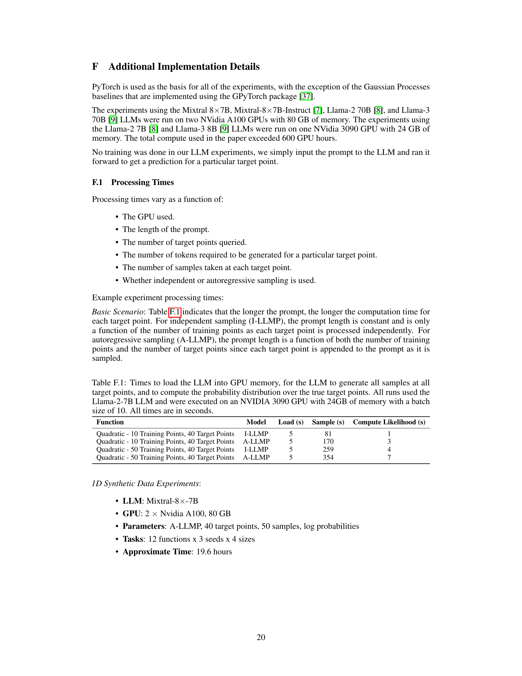
This table shows the time it takes to load the Llama-2-7B LLM into GPU memory, generate samples for all target points using the LLM, and compute likelihoods for the true target points. The experiment used an NVIDIA 3090 GPU with 24GB memory and a batch size of 10. Times are reported in seconds and vary based on the number of training points and whether independent or autoregressive sampling is used.

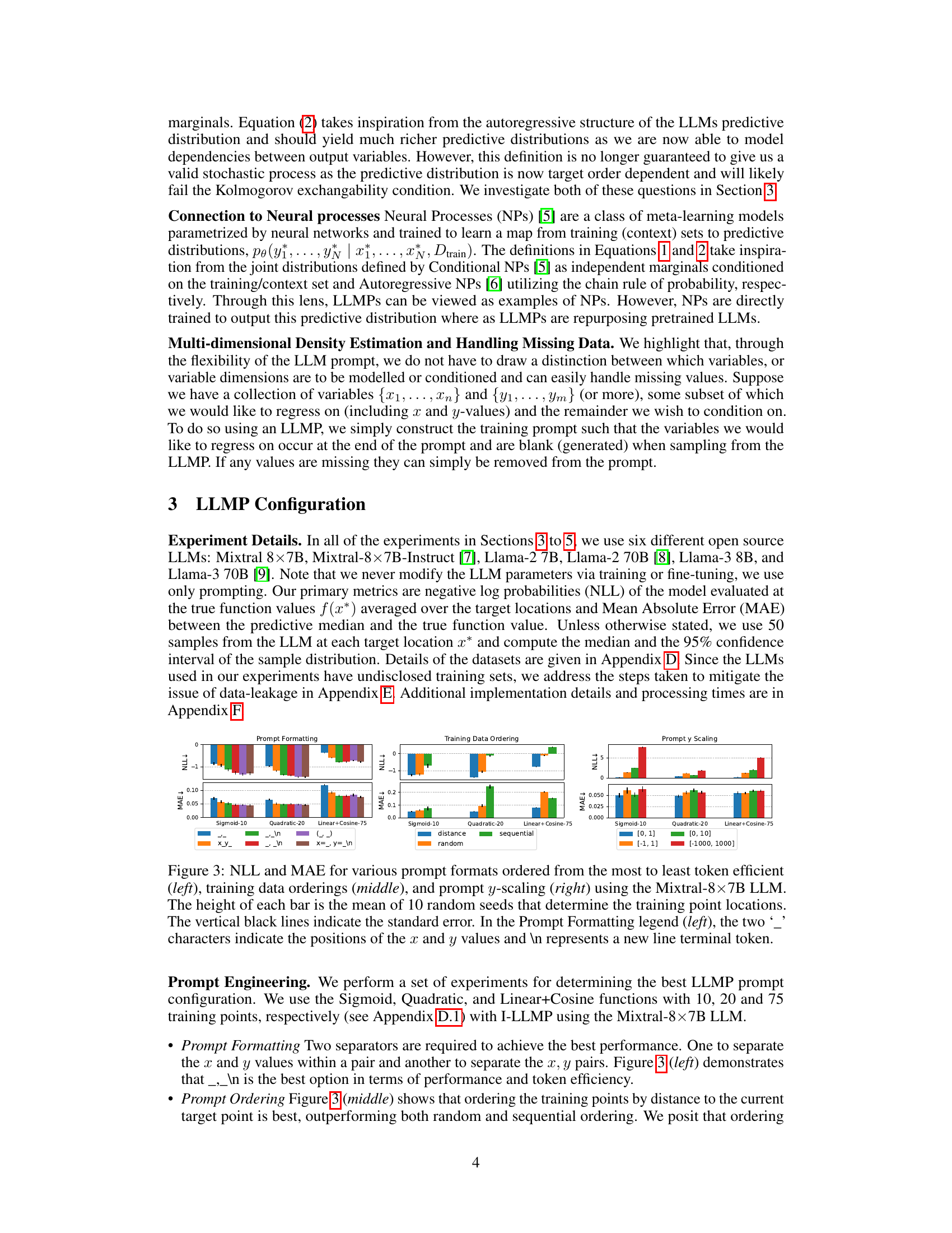
This table presents the negative log-likelihood (NLL) and Mean Absolute Error (MAE) for different prompt formats across three large language models (LLMs). The results are averaged over multiple random seed initializations, each determining the positions of observed data points. The table shows how different formatting schemes for the prompt affect the LLMs’ performance on various functions with varying numbers of observed points. It is organized to demonstrate the effect of prompt structure on model accuracy.

This table shows the negative log-likelihood (NLL) and mean absolute error (MAE) for different prompt formats used with three different large language models (LLMs). Each bar represents the average performance over ten different random seed configurations, indicating the variation in results. The prompt formats are compared based on their token efficiency. The most efficient format is indicated on the left, while the least efficient is on the right.

This table shows the results of an experiment comparing three different training data orderings for LLMs: sequential, random, and distance-based. The table presents the mean average error (MAE) and negative log-likelihood (NLL) for each ordering across three different LLMs (Llama-2-7B, Llama-2-70B, and Mixtral-8x7B) on three synthetic function datasets (Sigmoid with 10 points, Quadratic with 20 points, and Linear + Cosine with 75 points). The distance-based ordering consistently shows the best results, likely because it emphasizes the relevance of data points closer to the prediction target.

This table presents a comparison of the Mean Absolute Error (MAE) and Negative Log-Likelihood (NLL) achieved by the Mixtral-8x7B A-LLMP model and a Gaussian Process (GP) model using a Radial Basis Function (RBF) kernel. The comparison is performed across seven different training set sizes (5, 10, 15, 20, 25, 50, and 75 data points) and three random seeds for each function. The results illustrate the predictive performance of both models on several synthetic functions and highlight how performance changes as the amount of training data varies.

This table presents a comparison of the Mean Absolute Error (MAE) and Negative Log-Likelihood (NLL) achieved by the Mixtral-8x7B A-LLMP model and a Gaussian Process (GP) model using a Radial Basis Function (RBF) kernel. The comparison is made across seven different training set sizes (5, 10, 15, 20, 25, 50, and 75 training points) for twelve different synthetic functions. The results are averaged across three random seeds for each function and training set size. The table aims to demonstrate the competitive performance of the LLMP model compared to a well-established GP regression model.

This table presents the results of an experiment comparing two methods for defining joint predictive distributions over multiple target locations (I-LLMP and A-LLMP) and using three different LLMs. The table shows the Mean Average Error (MAE) and Negative Log Likelihood (NLL) for each method, with the training data ordered randomly or by distance to the target point. The results indicate that the autoregressive approach (A-LLMP) generally achieves better performance, particularly when using distance-ordered training data.

This table compares the performance of Optuna and Llama-7B in a black-box optimization task across six different functions with varying numbers of dimensions. For each function, it shows the true maximum value, the trial number at which the best result was achieved by each method, and the best maximum value found by each method. This allows for a comparison of the efficiency and effectiveness of each method in finding the optimum.
Full paper#


