TL;DR#
Predicting neural network properties solely from their weights is challenging due to the vast diversity in network architectures and parameter sizes. Existing methods often require architecture-specific models, limiting their applicability and generalizability. They also neglect the hierarchical structure inherent in many networks.
The proposed Set-based Neural Network Encoder (SNE) addresses these issues by using set-to-set and set-to-vector functions to encode network weights efficiently and in an architecture-agnostic manner. SNE considers the hierarchical structure of networks during encoding and employs Logit Invariance to ensure minimal invariance properties. This approach, coupled with a pad-chunk-encode pipeline, allows it to handle neural networks of arbitrary size and architecture. Evaluation shows SNE outperforms existing baselines in standard benchmarks and on newly introduced tasks evaluating cross-dataset and cross-architecture generalization. SNE’s architecture-agnostic nature and improved generalizability represent significant advancements in neural network analysis and property prediction.
Key Takeaways#
Why does it matter?#
This paper is crucial because it introduces a novel and efficient method for encoding neural network weights, enabling property prediction across diverse architectures and datasets. This addresses a critical limitation of existing methods and opens new avenues for research in model analysis and transfer learning. The method’s ability to handle varying network sizes and structures makes it highly relevant to current deep learning research trends, pushing the boundaries of efficient model analysis and application. Its introduction of new tasks for evaluating model generalization further enhances its value to the community.
Visual Insights#

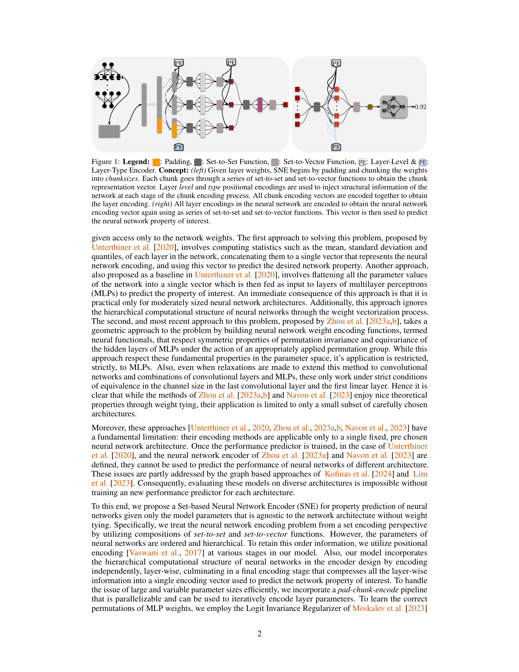
🔼 This figure illustrates the architecture of the Set-based Neural Network Encoder (SNE). The left panel shows how SNE processes individual layers: weights are padded and chunked, each chunk is processed by set functions to produce a chunk representation, layer positional encodings are added, and all chunk representations are combined into a layer encoding. The right panel shows how these layer encodings are combined to get a final neural network encoding that is used for predicting the network’s properties. The figure uses visual cues (color-coding, shapes) to represent different steps and components in the SNE process.
read the caption
Figure 1: Legend: : Padding, : Set-to-Set Function, : Set-to-Vector Function, PE: Layer-Level & Layer-Type Encoder. Concept: (left) Given layer weights, SNE begins by padding and chunking the weights into chunksizes. Each chunk goes through a series of set-to-set and set-to-vector functions to obtain the chunk representation vector. Layer level and type positional encodings are used to inject structural information of the network at each stage of the chunk encoding process. All chunk encoding vectors are encoded together to obtain the layer encoding. (right) All layer encodings in the neural network are encoded to obtain the neural network encoding vector again using as series of set-to-set and set-to-vector functions. This vector is then used to predict the neural network property of interest.
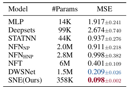
🔼 This table presents the results of predicting the frequencies of Implicit Neural Representations (INRs). It compares the performance of several models (MLP, Deepsets, STATNN, NFNNP, NFNHNP, NFT, DWSNet, and the proposed SNE model) on this task by showing the number of parameters (#Params) and the Mean Squared Error (MSE) achieved by each model. The MSE is a measure of how well the model predicts the frequency, with lower values indicating better performance. The table highlights that SNE significantly outperforms other baselines.
read the caption
Table 1: Predicting Frequencies of Implicit Neural Representations (INRs).
In-depth insights#
Set Encoding#
The concept of ‘Set Encoding’ in the context of neural network weight encoding is crucial. It addresses the challenge of handling the inherent unordered nature of neural network parameters. Traditional methods often flatten weights, losing structural information. Set-based approaches, however, acknowledge the set-like properties of these parameters. This allows for the development of encoding techniques robust to permutations, respecting the symmetries within the weight space. The effectiveness of set encoding hinges on the choice of set functions (such as Set-to-Set and Set-to-Vector functions) that capture both intra-set and inter-set relationships. This approach is particularly valuable when dealing with varied network architectures, because it offers architecture-agnostic encoding. By incorporating positional encodings or other mechanisms to retain order information, set-based methods strive for efficient and informative representations of neural network weights, facilitating property prediction and other tasks. The success of set encoding depends on skillful design of these functions and consideration of any inherent hierarchical structure within the network itself. This is crucial for accurate encoding that captures the true essence of the underlying network. The advantages become evident when comparing it to flattening, a crude method that is clearly less informative.
SNE#
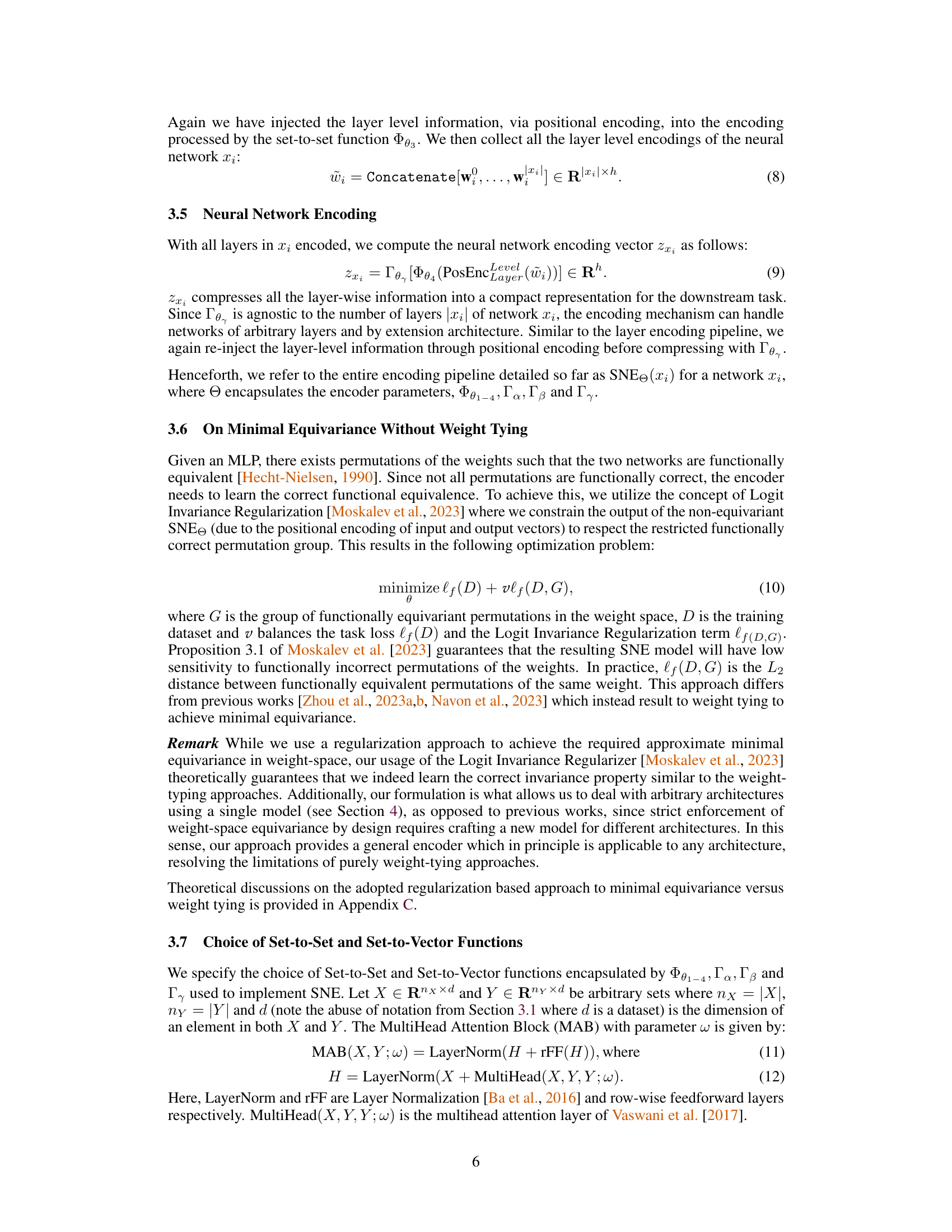
The Set-based Neural Network Encoder (SNE) is a novel method for encoding neural network weights, agnostic to the network’s architecture. This is a significant improvement over existing methods that require custom encoders for different architectures. SNE leverages set-to-set and set-to-vector functions, effectively handling the hierarchical structure of neural networks and addressing weight symmetries using Logit Invariance. The pad-chunk-encode pipeline enhances efficiency by processing large weight tensors in parallel. SNE’s architecture-agnostic nature allows it to generalize across datasets and architectures, outperforming baselines in cross-dataset and cross-architecture property prediction tasks. Its ability to handle arbitrary architectures represents a key advancement in neural network property prediction, paving the way for more versatile and robust applications. While weight-tying methods enjoy strong theoretical guarantees, SNE instead uses a regularization approach, offering similar performance with greater flexibility.
Cross-Dataset#
The heading ‘Cross-Dataset’ suggests an experimental design evaluating the generalizability of a model trained on one dataset to other, unseen datasets. This is crucial for assessing robustness and real-world applicability. A successful cross-dataset evaluation demonstrates that the model isn’t overfitting to specific dataset biases, and its learned features transfer effectively to diverse data distributions. The results of this section will likely showcase the model’s ability to generalize across variations in data characteristics (noise levels, sample sizes, data collection methods, etc.), providing important insights into its performance in novel and potentially challenging situations. A strong cross-dataset performance would indicate a model more likely to be deployed effectively in practical settings where data characteristics may vary.
Cross-Arch#
The heading ‘Cross-Arch’, likely short for ‘Cross-Architecture’, signifies a crucial experimental design in evaluating neural network property prediction models. It focuses on the model’s ability to generalize across unseen architectures, testing its robustness beyond the specific network structures used for training. This is a significant step towards creating truly versatile and practical predictors, as real-world scenarios rarely involve only one architecture. Successfully navigating the ‘Cross-Arch’ challenge demonstrates architecture-agnostic learning, a desirable characteristic for broader applicability. The results from this section would reveal if the model captures fundamental properties of neural networks that are transferable across different designs, or if it overfits to the specific architecture in the training data. A strong ‘Cross-Arch’ performance indicates a deeper understanding of neural network behavior, while poor performance suggests an over-reliance on training data specifics. This is a key differentiator between shallow statistical analysis and genuinely insightful neural network encoding methods.
Limitations#
The limitations section of a research paper is crucial for demonstrating critical thinking and acknowledging the boundaries of the study. A thoughtful limitations section should address the scope of the claims, honestly acknowledging the contexts in which the findings might not generalize. This often involves discussing assumptions made during the research process and the robustness of the findings to violations of these assumptions, such as data limitations or model simplifications. For example, a study relying on a specific dataset might note the potential impact of dataset bias on the conclusions. A limitations section should also address methodological limitations, such as constraints on sample size or the use of specific statistical techniques. The discussion should assess potential limitations on the generalizability of the results, including limitations related to the study population or setting, and how these factors might affect the interpretation of the findings. Finally, the limitations section can suggest directions for future research. Clearly articulating limitations enhances the credibility of the research by demonstrating awareness of the study’s boundaries and suggesting avenues for future work.
More visual insights#
More on figures

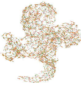
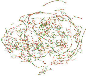
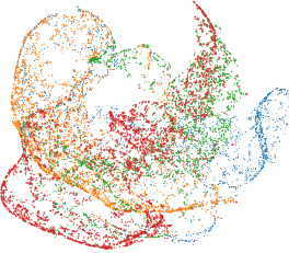
🔼 This figure shows the t-distributed stochastic neighbor embedding (t-SNE) visualizations of neural network encodings generated by different methods (MLP, STATNN, NFNNP, NFNHNP, and SNE) trained on a combination of four model zoos (MNIST, FashionMNIST, CIFAR10, and SVHN). The visualizations illustrate how well each method separates the neural networks from different datasets in a 3D embedding space. The caption indicates that larger versions are available in Appendix K, highlighting the detail in the visualizations that might be hard to see in this reduced version.
read the caption
Figure 2: TSNE Visualization of Neural Network Encodings. We train neural network performance prediction methods on a combination of the MNIST, FashionMNIST, CIFAR10 and SVHN modelzoos of Unterthiner et al. [2020]. We present 3 views of the resulting 3-D plots showing how neural networks from each modelzoo are embedded/encoded by the corresponding models. Larger versions of these figures are provided in Appendix K. Zoom in for better viewing.
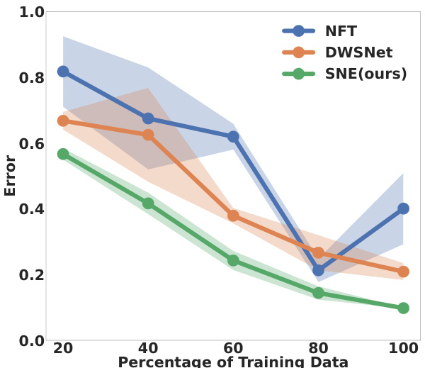
🔼 The figure shows the performance of three neural network encoding methods (NFT, DWSNet, and SNE) under different amounts of training data. The x-axis represents the percentage of the training data used, and the y-axis represents the error rate. The shaded areas around the lines represent confidence intervals. The plot demonstrates that SNE is more data-efficient than the other methods, maintaining lower error rates even with a smaller percentage of training data.
read the caption
Figure 3: Ablation: We compare the performance of models in a limited training data setting using the experiments of Table 1. As shown, SNE is more data efficient than the baseline models when the amount of training data is constrained.

🔼 This figure shows t-SNE visualizations of neural network encodings generated by different methods (MLP, STATNN, NFNNP, NFNHNP, and SNE) trained on a combination of MNIST, FashionMNIST, CIFAR10, and SVHN datasets. The plots illustrate how well each method separates the neural networks from different datasets in the latent space. The SNE method shows a more uniform distribution indicating its better generalization across different model zoos. Appendix K provides larger versions of these plots for more detailed viewing.
read the caption
Figure 2: TSNE Visualization of Neural Network Encodings. We train neural network performance prediction methods on a combination of the MNIST, FashionMNIST, CIFAR10 and SVHN modelzoos of Unterthiner et al. [2020]. We present 3 views of the resulting 3-D plots showing how neural networks from each modelzoo are embedded/encoded by the corresponding models. Larger versions of these figures are provided in Appendix K. Zoom in for better viewing.

🔼 This figure shows t-SNE visualizations of neural network encodings generated by different methods (MLP, STATNN, NFNNP, NFNHNP, and SNE) trained on a combination of MNIST, FashionMNIST, CIFAR10, and SVHN model zoos. The visualizations illustrate how well each method separates neural networks from different datasets in a 3D embedding space. Larger versions of these plots are available in Appendix K.
read the caption
Figure 2: TSNE Visualization of Neural Network Encodings. We train neural network performance prediction methods on a combination of the MNIST, FashionMNIST, CIFAR10 and SVHN modelzoos of Unterthiner et al. [2020]. We present 3 views of the resulting 3-D plots showing how neural networks from each modelzoo are embedded/encoded by the corresponding models. Larger versions of these figures are provided in Appendix K. Zoom in for better viewing.
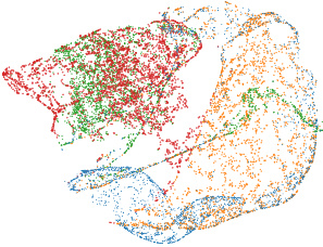
🔼 This figure shows the t-SNE visualization of neural network encodings generated by different methods (MLP, STATNN, NFNNP, NFNHNP, and SNE). Each point represents a neural network from one of four model zoos (MNIST, FashionMNIST, CIFAR10, and SVHN). The visualization helps to understand how well each encoding method separates networks from different datasets and its ability to generalize across datasets.
read the caption
Figure 2: TSNE Visualization of Neural Network Encodings. We train neural network performance prediction methods on a combination of the MNIST, FashionMNIST, CIFAR10 and SVHN modelzoos of Unterthiner et al. [2020]. We present 3 views of the resulting 3-D plots showing how neural networks from each modelzoo are embedded/encoded by the corresponding models. Larger versions of these figures are provided in Appendix K. Zoom in for better viewing.

🔼 This figure shows t-SNE visualizations of neural network encodings generated by different models (MLP, STATNN, NFNNP, NFNHNP, and SNE) trained on a combined dataset of MNIST, FashionMNIST, CIFAR10, and SVHN. The visualizations illustrate how well each model separates neural networks from different datasets in a three-dimensional embedding space. The plots aim to show differences in the ability of the methods to learn meaningful representations of the network weights, highlighting the distinct performance of SNE (the proposed model) compared to others.
read the caption
Figure 2: TSNE Visualization of Neural Network Encodings. We train neural network performance prediction methods on a combination of the MNIST, FashionMNIST, CIFAR10 and SVHN modelzoos of Unterthiner et al. [2020]. We present 3 views of the resulting 3-D plots showing how neural networks from each modelzoo are embedded/encoded by the corresponding models. Larger versions of these figures are provided in Appendix K. Zoom in for better viewing.

🔼 This figure shows t-SNE visualizations of neural network encodings generated by different methods (MLP, STATNN, NFNNP, NFNHNP, and SNE). Each point represents a neural network from one of four model zoos (MNIST, FashionMNIST, CIFAR10, and SVHN). The plots illustrate how well each method separates networks from different datasets and how this relates to the methods’ performance on cross-dataset generalization.
read the caption
Figure 2: TSNE Visualization of Neural Network Encodings. We train neural network performance prediction methods on a combination of the MNIST, FashionMNIST, CIFAR10 and SVHN modelzoos of Unterthiner et al. [2020]. We present 3 views of the resulting 3-D plots showing how neural networks from each modelzoo are embedded/encoded by the corresponding models. Larger versions of these figures are provided in Appendix K. Zoom in for better viewing.

🔼 This figure shows t-SNE visualizations of neural network encodings generated by different methods (MLP, STATNN, NFNNP, NFNHNP, and SNE) trained on a combination of MNIST, FashionMNIST, CIFAR10, and SVHN model zoos. The visualizations illustrate how well each method separates neural networks from different datasets in a 3D embedding space. The goal is to show how the various methods perform in terms of clustering networks from the same source together, with SNE ideally showing tight clusters of networks from the same dataset.
read the caption
Figure 2: TSNE Visualization of Neural Network Encodings. We train neural network performance prediction methods on a combination of the MNIST, FashionMNIST, CIFAR10 and SVHN modelzoos of Unterthiner et al. [2020]. We present 3 views of the resulting 3-D plots showing how neural networks from each modelzoo are embedded/encoded by the corresponding models. Larger versions of these figures are provided in Appendix K. Zoom in for better viewing.

🔼 This figure shows t-SNE visualizations of neural network encodings generated by different methods (MLP, STATNN, NFNNP, NFNHNP, and SNE) trained on a combination of MNIST, FashionMNIST, CIFAR10, and SVHN model zoos. The visualizations illustrate how well each method separates the encodings from different datasets, providing insights into the effectiveness of each encoding technique in capturing the essential properties of the neural networks.
read the caption
Figure 2: TSNE Visualization of Neural Network Encodings. We train neural network performance prediction methods on a combination of the MNIST, FashionMNIST, CIFAR10 and SVHN modelzoos of Unterthiner et al. [2020]. We present 3 views of the resulting 3-D plots showing how neural networks from each modelzoo are embedded/encoded by the corresponding models. Larger versions of these figures are provided in Appendix K. Zoom in for better viewing.
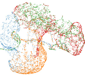
🔼 This figure shows t-SNE visualizations of neural network encodings generated by different methods (MLP, STATNN, NFNNP, NFNHNP, and SNE) trained on a combination of MNIST, FashionMNIST, CIFAR10, and SVHN model zoos. The visualizations illustrate how well each method clusters neural networks from the same dataset, revealing differences in the methods’ ability to capture relevant information about the network architectures and training data.
read the caption
Figure 2: TSNE Visualization of Neural Network Encodings. We train neural network performance prediction methods on a combination of the MNIST, FashionMNIST, CIFAR10 and SVHN modelzoos of Unterthiner et al. [2020]. We present 3 views of the resulting 3-D plots showing how neural networks from each modelzoo are embedded/encoded by the corresponding models. Larger versions of these figures are provided in Appendix K. Zoom in for better viewing.

🔼 This figure shows t-SNE visualizations of neural network encodings generated by different methods (MLP, STATNN, NFNNP, NFNHNP, and SNE). The methods were trained on a combined dataset of MNIST, Fashion-MNIST, CIFAR-10, and SVHN. The visualizations illustrate how these methods group the neural networks from each dataset in a 3D embedding space. SNE’s embedding shows a more uniform distribution of networks across datasets, suggesting better generalization across different datasets compared to the other methods. The full versions of the plots shown here are in Appendix K.
read the caption
Figure 2: TSNE Visualization of Neural Network Encodings. We train neural network performance prediction methods on a combination of the MNIST, FashionMNIST, CIFAR10 and SVHN modelzoos of Unterthiner et al. [2020]. We present 3 views of the resulting 3-D plots showing how neural networks from each modelzoo are embedded/encoded by the corresponding models. Larger versions of these figures are provided in Appendix K. Zoom in for better viewing.
🔼 This figure shows t-SNE visualizations of neural network encodings generated by different models (MLP, STATNN, NFNNP, NFNHNP, and SNE) trained on a combined dataset of MNIST, FashionMNIST, CIFAR10, and SVHN. The visualizations illustrate how each model represents the relationships between different neural network architectures from those datasets. The goal is to observe how well each model clusters networks from the same dataset and separates them from other datasets, demonstrating the effectiveness of the encoding methods in capturing and preserving relevant information about the neural networks’ properties.
read the caption
Figure 2: TSNE Visualization of Neural Network Encodings. We train neural network performance prediction methods on a combination of the MNIST, FashionMNIST, CIFAR10 and SVHN modelzoos of Unterthiner et al. [2020]. We present 3 views of the resulting 3-D plots showing how neural networks from each modelzoo are embedded/encoded by the corresponding models. Larger versions of these figures are provided in Appendix K. Zoom in for better viewing.

🔼 This figure shows t-SNE visualizations of neural network encodings generated by different methods (MLP, STATNN, NFNNP, NFNHNP, and SNE). Each point represents a neural network from one of four model zoos (MNIST, FashionMNIST, CIFAR10, and SVHN), and the color indicates the dataset. The visualization helps to understand how well each method separates networks from different datasets, showing SNE has the best separation.
read the caption
Figure 2: TSNE Visualization of Neural Network Encodings. We train neural network performance prediction methods on a combination of the MNIST, FashionMNIST, CIFAR10 and SVHN modelzoos of Unterthiner et al. [2020]. We present 3 views of the resulting 3-D plots showing how neural networks from each modelzoo are embedded/encoded by the corresponding models. Larger versions of these figures are provided in Appendix K. Zoom in for better viewing.
🔼 This figure shows t-SNE visualizations of neural network encodings generated by different methods (MLP, STATNN, NFNNP, NFNHNP, and SNE) trained on a combined dataset of MNIST, FashionMNIST, CIFAR10, and SVHN. The visualizations illustrate how well each method separates neural networks from different datasets in the latent space, highlighting the effectiveness of SNE in generating similar embeddings for networks from various datasets.
read the caption
Figure 2: TSNE Visualization of Neural Network Encodings. We train neural network performance prediction methods on a combination of the MNIST, FashionMNIST, CIFAR10 and SVHN modelzoos of Unterthiner et al. [2020]. We present 3 views of the resulting 3-D plots showing how neural networks from each modelzoo are embedded/encoded by the corresponding models. Larger versions of these figures are provided in Appendix K. Zoom in for better viewing.
🔼 This figure shows t-SNE visualizations of neural network encodings produced by different methods (MLP, STATNN, NFNNP, NFNHNP, and SNE). Each point represents a neural network from one of four datasets (MNIST, FashionMNIST, CIFAR10, and SVHN). The plots illustrate how well each encoding method separates neural networks from different datasets. SNE shows a more uniform distribution, indicating better generalization across datasets.
read the caption
Figure 2: TSNE Visualization of Neural Network Encodings. We train neural network performance prediction methods on a combination of the MNIST, FashionMNIST, CIFAR10 and SVHN modelzoos of Unterthiner et al. [2020]. We present 3 views of the resulting 3-D plots showing how neural networks from each modelzoo are embedded/encoded by the corresponding models. Larger versions of these figures are provided in Appendix K. Zoom in for better viewing.

🔼 This figure shows t-SNE visualizations of neural network encodings generated by different methods (MLP, STATNN, NFNNP, NFNHNP, and SNE). Each point represents a neural network from one of four datasets (MNIST, FashionMNIST, CIFAR10, and SVHN). The plots illustrate how well the different encoding methods separate neural networks from different datasets. SNE demonstrates a more uniform embedding of networks across datasets, suggesting better generalization.
read the caption
Figure 2: TSNE Visualization of Neural Network Encodings. We train neural network performance prediction methods on a combination of the MNIST, FashionMNIST, CIFAR10 and SVHN modelzoos of Unterthiner et al. [2020]. We present 3 views of the resulting 3-D plots showing how neural networks from each modelzoo are embedded/encoded by the corresponding models. Larger versions of these figures are provided in Appendix K. Zoom in for better viewing.

🔼 This figure shows t-SNE visualizations of neural network encodings generated by different methods (MLP, STATNN, NFNNP, NFNHNP, and SNE). The models were trained on a combined dataset of MNIST, FashionMNIST, CIFAR10, and SVHN. Each point represents a single neural network, and the color indicates the dataset the network was trained on. The visualization aims to illustrate how effectively each encoding method separates networks trained on different datasets and reveals patterns in the relationships between different network encodings. The figure indicates that SNE produces more homogeneous embedding across datasets, while the other methods show distinct clusters for different datasets.
read the caption
Figure 2: TSNE Visualization of Neural Network Encodings. We train neural network performance prediction methods on a combination of the MNIST, FashionMNIST, CIFAR10 and SVHN modelzoos of Unterthiner et al. [2020]. We present 3 views of the resulting 3-D plots showing how neural networks from each modelzoo are embedded/encoded by the corresponding models. Larger versions of these figures are provided in Appendix K. Zoom in for better viewing.
More on tables
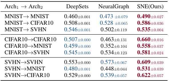
🔼 This table presents the results of the cross-architecture performance prediction task. It demonstrates the generalization performance of the encoder trained on three homogeneous model zoos of the same architecture when tested on three different architectures unseen during training. The rows represent the source architecture and target architecture used for training and testing, respectively. The columns show the performance of different neural network encoding methods (DeepSets, NeuralGraph, and SNE). The results show how well the performance predictors transfer to unseen architectures. The model zoos are trained on MNIST, CIFAR10, and SVHN datasets.
read the caption
Table 2: Cross-Architecture Performance Prediction.

🔼 This table presents the results of the cross-architecture performance prediction task on the model zoo of Schürholt et al. [2022]. It demonstrates how well the SNE model generalizes to unseen architectures. The table compares the performance of SNE and HyperRep on three different cross-architecture transfer tasks, where models are trained on SVHN and tested on SVHN, MNIST, and CIFAR10, respectively. The results show that SNE significantly outperforms HyperRep in all three scenarios, indicating that SNE is more robust in handling unseen architectures compared to HyperRep.
read the caption
Table 3: Cross-Architecture Performance Prediction on Schürholt et al. [2022]'s model zoo.

🔼 This table presents the results of cross-architecture performance prediction on transformers. The experiment evaluates how well performance predictors trained on a specific architecture (Arch1) transfer to an unseen architecture (Transformer). Three datasets (MNIST, CIFAR10, and SVHN) were used, and each dataset’s model zoo was used to evaluate the transfer performance from its associated Arch1 models to a transformer architecture trained on MNIST. The table shows the Kendall’s τ correlation values for each dataset and the two compared methods (DeepSets and SNE). SNE consistently outperforms DeepSets, demonstrating its better ability to generalize across unseen architectures.
read the caption
Table 4: Cross-Architecture Performance on Transformers. We report Kendall's τ.

🔼 This table presents the results of the cross-dataset performance prediction task. Kendall’s τ, a rank correlation measure, is used to evaluate the performance of different models. Each row represents a different cross-dataset evaluation scenario (e.g., MNIST to FashionMNIST). The table shows how well models trained on one dataset generalize to other unseen datasets. The best performing model for each row is highlighted in red, and the second best in blue.
read the caption
Table 5: Cross-Dataset Prediction. We report Kendall's τ.

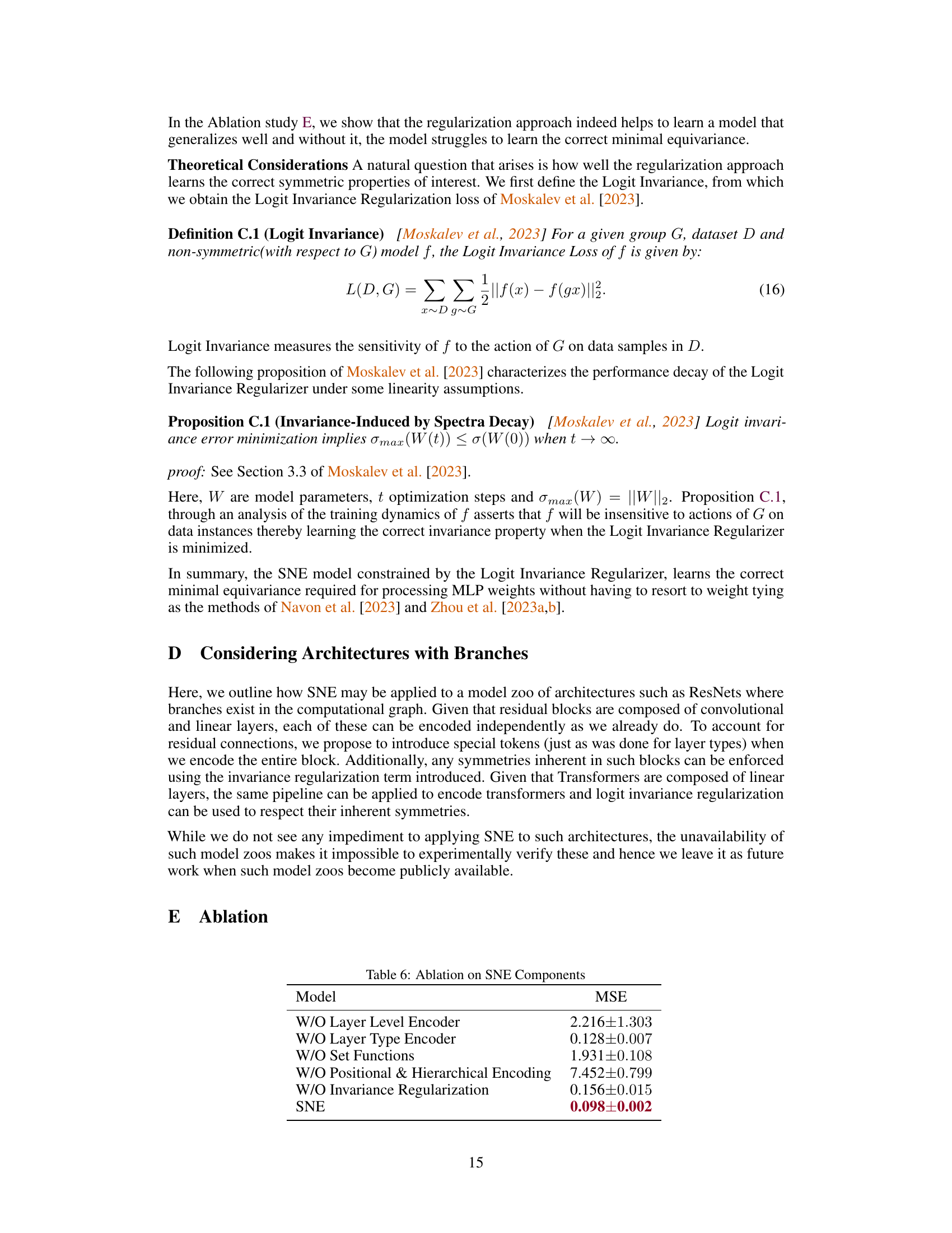
🔼 This ablation study analyzes the impact of different components of the Set-based Neural Network Encoder (SNE) on its performance. The results show the mean squared error (MSE) achieved by models missing various elements of the SNE, including the layer level encoder, layer type encoder, set functions, positional and hierarchical encoding, and the invariance regularization. The table highlights the contribution of each component to the overall performance, demonstrating the effectiveness of SNE’s design.
read the caption
Table 6: Ablation on SNE Components

🔼 This table presents an ablation study on the effect of different chunk sizes on the model’s performance. The chunk size is a hyperparameter that determines how the weights of each layer in the neural network are divided into smaller chunks for processing. The results show that the model’s performance (measured by MSE) is relatively stable across a range of chunk sizes, suggesting that the choice of chunk size may not be highly critical.
read the caption
Table 7: Effect of Chunksize.
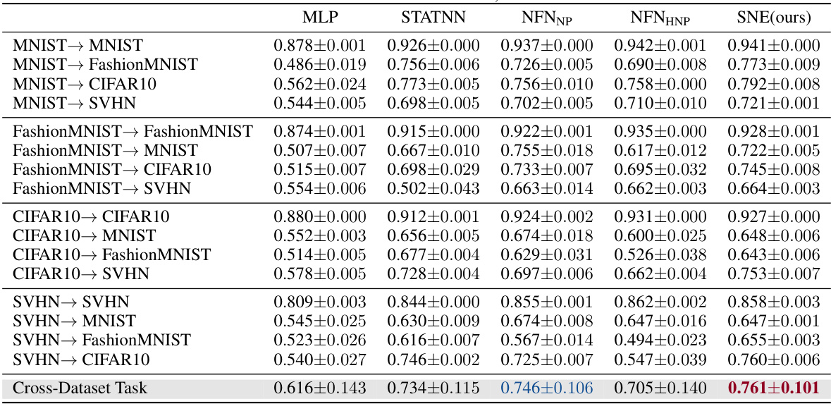
🔼 This table presents the results of a cross-dataset experiment, evaluating the performance of various methods in predicting neural network properties. Each method was trained on a model zoo from a single dataset (e.g., MNIST) and then tested on model zoos from other datasets (MNIST, FashionMNIST, CIFAR10, SVHN). The table shows the Kendall’s Tau correlation coefficient, measuring the rank correlation between predicted and actual properties. The best and second-best performing methods for each dataset combination are highlighted.
read the caption
Table 8: Cross-Dataset Neural Network Performance Prediction. We benchmark how well each method transfers across multiple datasets. In the first column, A → B implies that a model trained on a homogeneous model zoo of dataset A is evaluated on a homogeneous model zoo of dataset B. In the last row, we report the averaged performance of all methods across the cross-dataset task. For each row, the best model is shown in red and the second best in blue. Models are evaluated in terms of Kendall's T, a rank correlation measure.

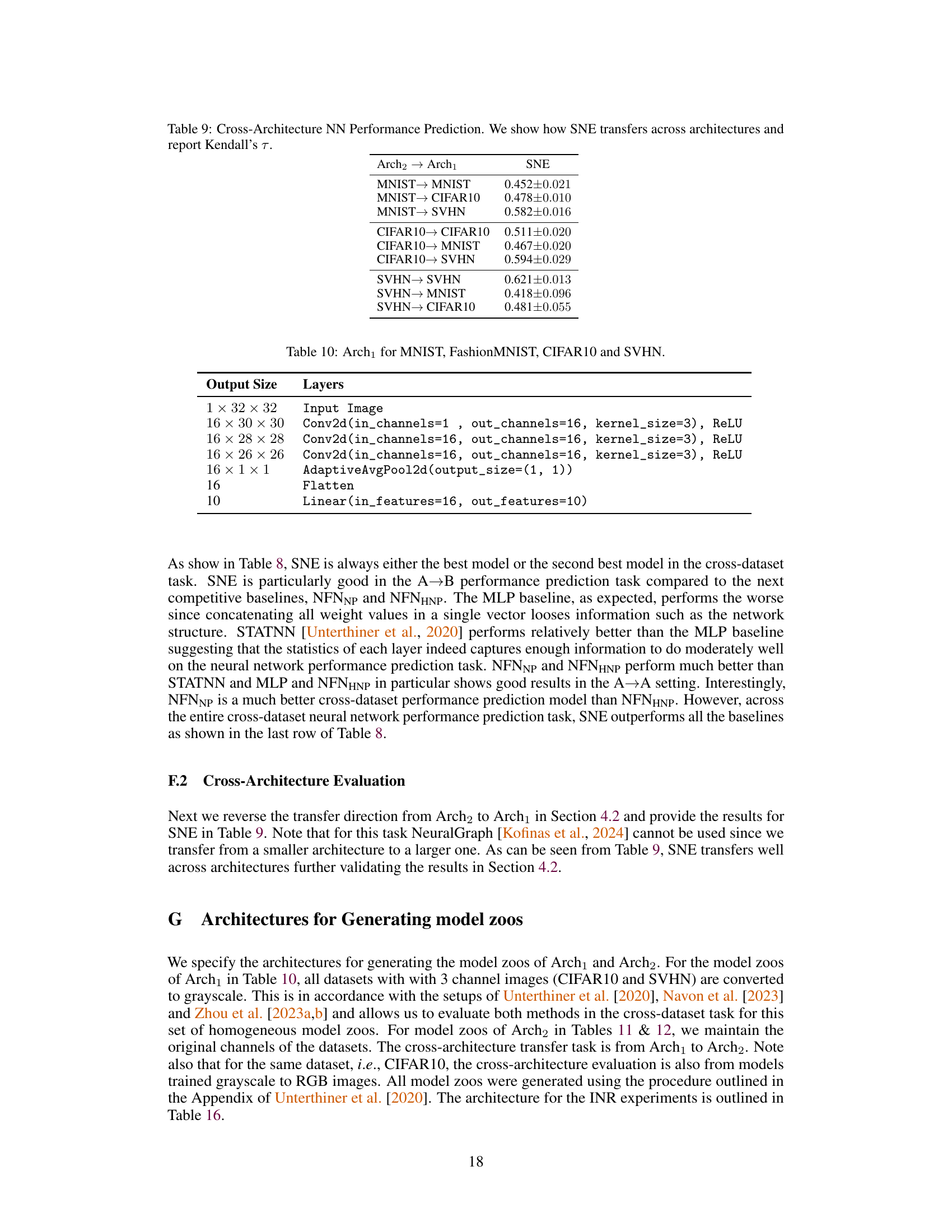
🔼 This table presents the results of the cross-architecture experiment. The experiment evaluates how well a neural network property predictor trained on a specific architecture generalizes to unseen architectures. Each row shows the Kendall’s τ (a rank correlation measure) for models trained on one architecture (Arch2) and tested on another (Arch1). The datasets used are MNIST, CIFAR10, and SVHN. The results demonstrate the ability of SNE to transfer across architectures.
read the caption
Table 9: Cross-Architecture NN Performance Prediction. We show how SNE transfers across architectures and report Kendall’s τ.

🔼 This table details the architecture used for generating the model zoos of Arch₁. Arch₁ is a specific architecture used in the cross-dataset and cross-architecture experiments described in the paper. The architecture consists of three convolutional layers, an adaptive average pooling layer, a flatten layer, and two linear layers, resulting in a 10-dimensional output. The input image sizes and channel specifications vary based on the dataset (MNIST, FashionMNIST, CIFAR10, and SVHN).
read the caption
Table 10: Arch₁ for MNIST, FashionMNIST, CIFAR10 and SVHN.

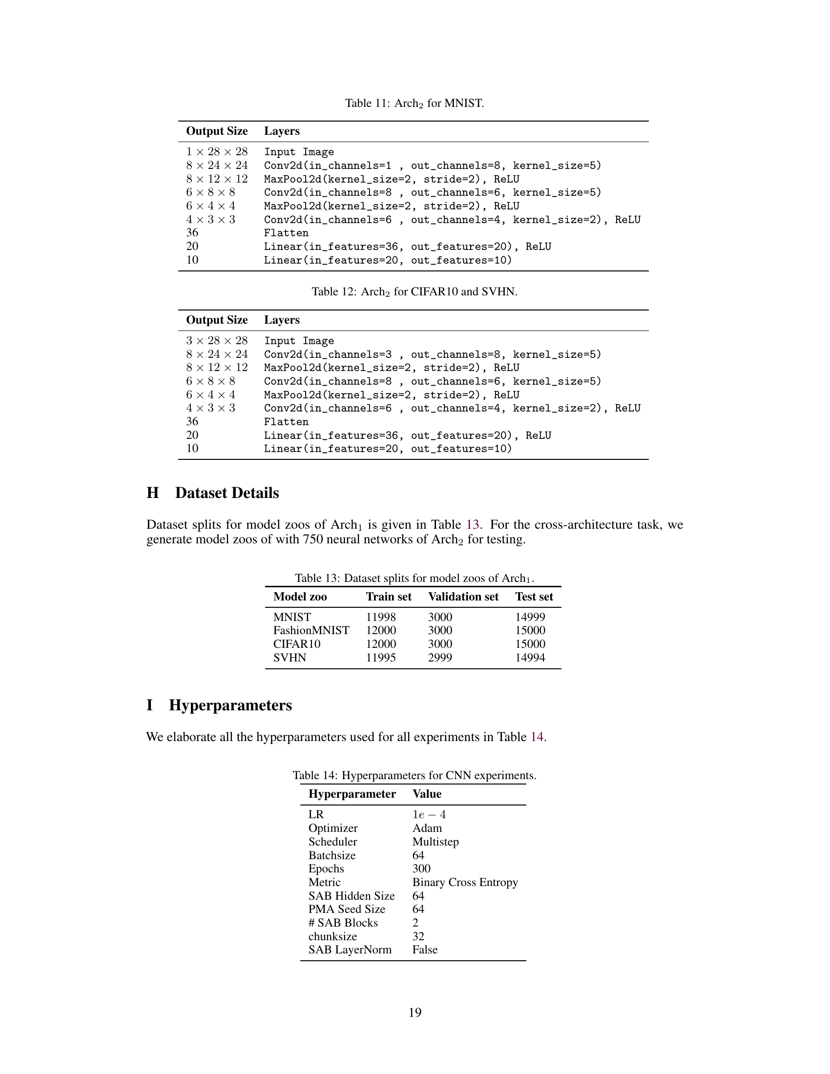
🔼 This table details the architecture of model zoos for the cross-architecture task, specifically for the MNIST dataset. It shows the layer-by-layer specifications including input size, number of channels, kernel size, activation function (ReLU), and max pooling. The final layers are linear layers leading to an output size of 10.
read the caption
Table 11: Arch2 for MNIST.

🔼 This table presents the architecture used for generating the model zoos of Arch2 for CIFAR10 and SVHN datasets in the cross-architecture experiments. It details the layers, their output sizes, and the operations involved for each layer in the architecture. The architecture consists of multiple convolutional layers, max-pooling layers, a flattening layer, and finally two linear layers to produce the output.
read the caption
Table 12: Arch2 for CIFAR10 and SVHN.

🔼 This table shows the number of neural networks in the training, validation, and testing sets for each of the four datasets used to create the model zoos of Arch1. The datasets include MNIST, FashionMNIST, CIFAR10, and SVHN. Arch1 refers to a specific neural network architecture used in the paper’s experiments.
read the caption
Table 13: Dataset splits for model zoos of Arch1.
🔼 This table presents the ablation study of different components of the proposed Set-based Neural Network Encoder (SNE). It shows the impact of removing each component on the model’s performance in terms of Mean Squared Error (MSE). The components include the Layer Level Encoder, the Layer Type Encoder, Set Functions, Positional and Hierarchical Encoding, and the Invariance Regularization.
read the caption
Table 6: Ablation on SNE Components

🔼 This table shows the architecture of the Implicit Neural Representations (INRs) used in the experiments. It specifies the number of layers, input and output sizes, and activation function (sinusoidal) used for each layer in the INR model.
read the caption
Table 16: INR Architecture. Activations are Sinusoidal

🔼 This table shows the architecture of the Implicit Neural Representations (INRs) used in the experiments. The INR architecture consists of three linear layers. The first two layers have an output size of 32 and use a sinusoidal activation function. The final layer outputs a single value and uses no activation function.
read the caption
Table 16: INR Architecture. Activations are Sinusoidal
Full paper#
