TL;DR#
Predicting structural vibrations is crucial for reducing noise in various applications, but traditional numerical methods are computationally expensive. This creates a bottleneck in design optimization, especially for complex structures with high-frequency responses. This paper highlights the need for more efficient methods that can rapidly evaluate numerous designs.
The paper introduces a new deep learning benchmark dataset focused on vibrating plates with various geometries and parameters. The authors propose a novel network architecture, called Frequency-Query Operator (FQO), designed to predict vibration patterns. FQOs efficiently predicts these patterns by integrating operator learning principles. The model’s performance surpasses existing methods, demonstrating the potential of deep learning for speeding up simulations and facilitating design optimization.
Key Takeaways#
Why does it matter?#
This paper is crucial for researchers in vibroacoustics and mechanical engineering. It addresses the high computational cost of traditional numerical simulations for predicting structural vibrations by proposing a deep learning approach. The introduced benchmark dataset and evaluation metrics will greatly facilitate the development and comparison of novel methods, potentially accelerating design optimization in various noisy applications.
Visual Insights#
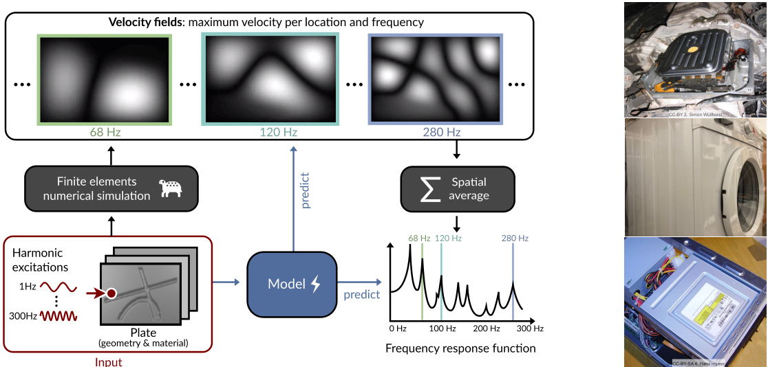
🔼 The figure shows the overall process of the proposed benchmark dataset. On the left, it displays how the dataset is created, starting from plate geometries and material properties, applying harmonic excitations, obtaining velocity fields through numerical simulations, and finally calculating the frequency response function. The right side illustrates the use of beadings in technical systems such as oil filters, washing machines, and disk drives. Beadings are indentations that alter the vibration patterns.
read the caption
Figure 1: Left: We introduce the Vibrating Plates dataset of 12,000 samples for predicting vibration patterns based on plate geometries. A harmonic force excites the plates, causing them to vibrate. The vibration patterns of the plates are obtained through numerical simulation. Diverse architectures are evaluated on the dataset. Right: Beadings are indentations and used in many vibrating technical systems. Here, on an oil filter, a washing machine and a disk drive. They increase the structural stiffness and alter the vibration.
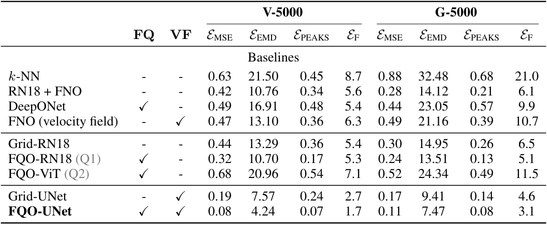
🔼 This table presents the performance of various machine learning models on the task of frequency response prediction. The models are evaluated using three metrics: Mean Squared Error (MSE), Earth Mover’s Distance (EEMD), and Peak Frequency Error (EPEAKS). The table also indicates whether each model uses a velocity field prediction (VF) and/or frequency queries (FQ) as part of its architecture. The results are shown separately for two dataset settings (V-5000 and G-5000).
read the caption
Table 1: Test results for frequency response prediction. Column VF indicates if F is indirectly predicted through the velocity field (Q3), column FQ indicates if frequency queries (Q1) are used. Q1 to Q3 refer to the model components described in Section 3.
In-depth insights#
Freq-Query Operator#
The proposed Freq-Query Operator (FQO) presents a novel neural network architecture designed for efficiently predicting the vibration patterns of plate geometries at specific excitation frequencies. Its key innovation lies in the integration of operator learning principles and implicit models for shape encoding. This approach cleverly addresses the challenge of predicting highly variable frequency response functions, common in dynamic systems. By directly querying the network for a specific frequency, FQO avoids the need for predicting the entire frequency spectrum, leading to significant computational efficiency gains. Implicit modeling allows for flexible predictions at any point in the frequency domain, even those unseen during training, showcasing a substantial advantage over grid-based methods. The method’s superior performance against existing approaches like DeepONets and Fourier Neural Operators further highlights its effectiveness and potential for applications in design optimization, which necessitates repeated calculations of vibrational behavior at various frequencies.
Vibrating Plates Data#
The “Vibrating Plates Data” section of this research paper is crucial as it forms the foundation for evaluating the proposed deep learning models for predicting structural vibrations. The dataset’s quality is paramount, and it appears to be meticulously constructed. The inclusion of 12,000 samples featuring varied plate geometries (including beadings), materials, boundary conditions, and excitation frequencies allows for a robust evaluation of model generalization capabilities. Furthermore, the dataset’s design considers practical engineering applications; the use of beadings is directly relevant to noise reduction techniques in real-world systems. The availability of associated numerical solutions (computed using FEM) allows for a quantitative assessment of the accuracy and efficiency of various deep learning models. This comparison is essential for demonstrating the potential of deep learning approaches as a faster alternative to traditional numerical simulations. The benchmark presented is therefore both comprehensive and practically relevant, contributing significantly to the advancement of deep learning methods in structural dynamics.
Deep Learning Models#
Deep learning has emerged as a powerful tool for modeling complex systems, and its application to predicting structural vibrations is a significant area of research. Surrogate models, trained on data from numerical simulations or experiments, offer the potential to significantly accelerate the design process compared to traditional computationally expensive methods like Finite Element Analysis (FEA). The choice of deep learning architecture is crucial; convolutional neural networks (CNNs) excel at processing spatial data, while recurrent neural networks (RNNs) are suitable for time-dependent phenomena. The selection should depend on the nature of the data and the specific problem being addressed; for example, predicting steady-state vibrations versus transient responses. Operator learning frameworks, like DeepONets and Fourier Neural Operators, are gaining traction for their ability to efficiently learn mappings between function spaces. These methods are particularly relevant for tasks involving high-dimensional inputs and outputs, such as those encountered when dealing with complex geometries and varying excitation frequencies. However, challenges remain, such as the need for substantial training datasets, handling of noisy data, and ensuring generalizability to unseen scenarios. Furthermore, integrating domain knowledge and physical constraints into the model architecture, for instance, using physics-informed neural networks, can improve accuracy and robustness.
Design Optimization#
The section on ‘Design Optimization’ explores the potential of using the Frequency-Query Operator (FQO)-UNet model for optimizing a plate’s design to reduce vibrations within a specific frequency range. This is a significant step beyond simple prediction, moving towards active design modification. The method combines a diffusion model for generating novel beading patterns with gradient information derived from the FQO-UNet. This gradient guides the diffusion process, driving it toward designs exhibiting reduced vibrations within the target frequency range. The results demonstrate that this approach is effective, producing plates with lower mean frequency responses in the targeted range than those found in the training dataset. This is a powerful demonstration of the model’s utility beyond basic prediction, showcasing its capacity for practical engineering applications such as noise reduction. Future work could involve exploring more complex geometries and material properties, further enhancing the model’s applicability to real-world engineering design challenges.
Future Work#
Future research directions stemming from this work could explore extending the model to handle more complex geometries beyond simple plates, such as curved shells or multi-component systems. This would necessitate developing more robust and flexible architectures capable of handling 3D data and diverse material properties. Another crucial area is improving sample efficiency; current methods require extensive FEM simulations. Investigating transfer learning techniques and developing more data-efficient deep learning architectures would significantly reduce computational costs. Furthermore, exploring the potential of this approach for practical design optimization tasks, such as noise reduction in complex systems, is a promising avenue for future work. Finally, a detailed analysis of the model’s sensitivity to different physical parameters and boundary conditions could enhance the understanding of its limitations and aid in the development of more robust and accurate surrogate models. This would involve a thorough investigation of error propagation and uncertainty quantification.
More visual insights#
More on figures

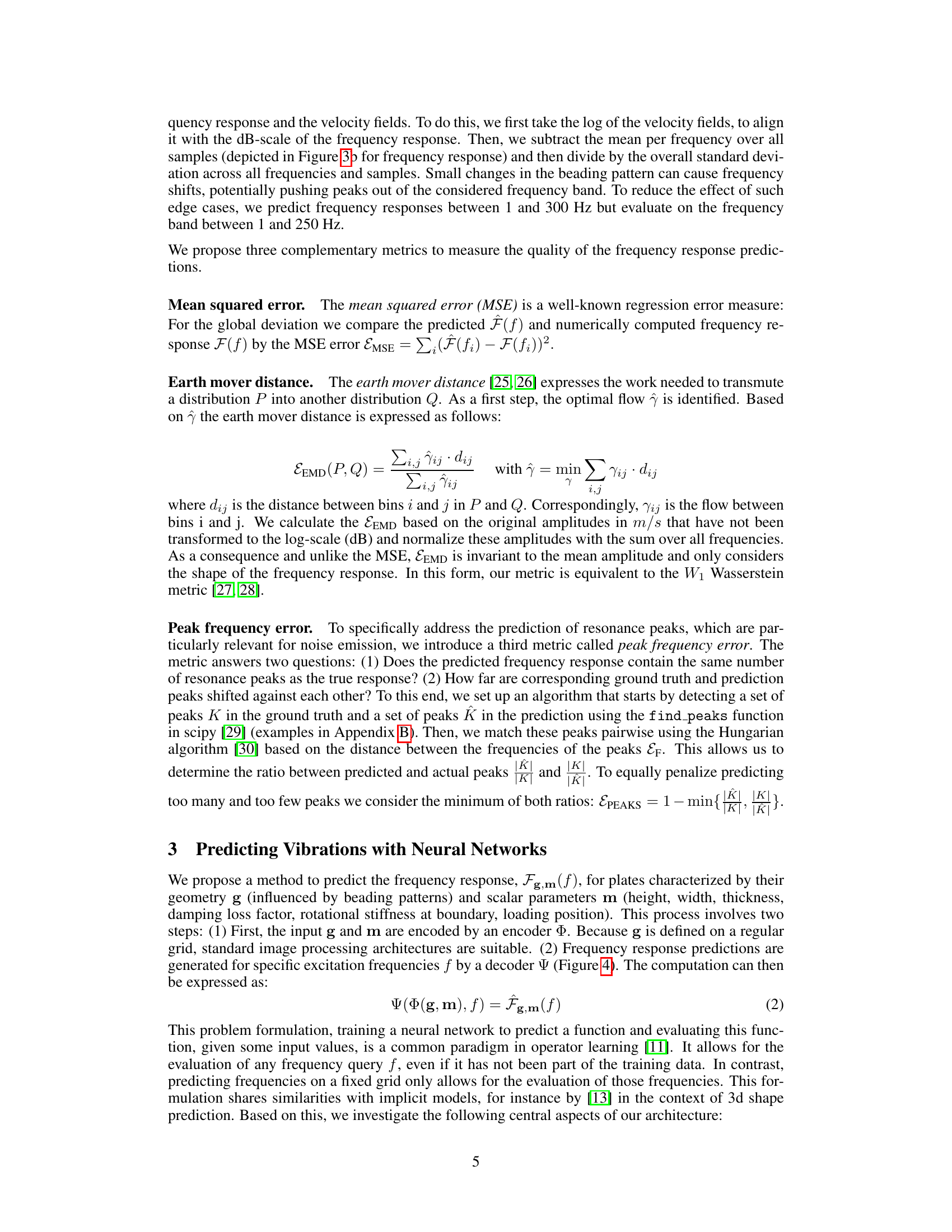
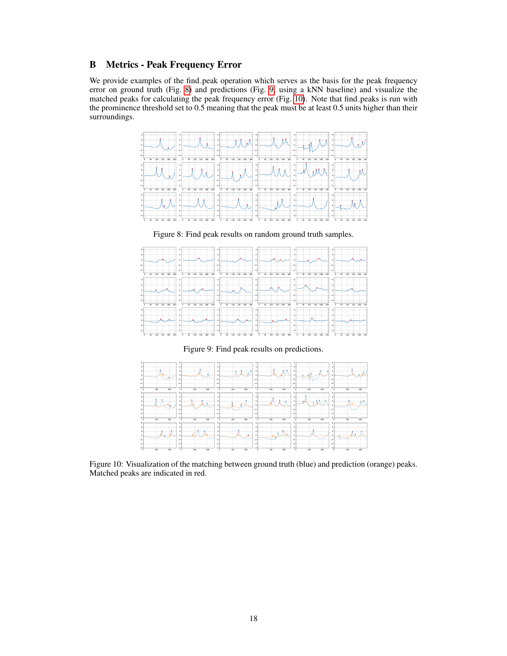
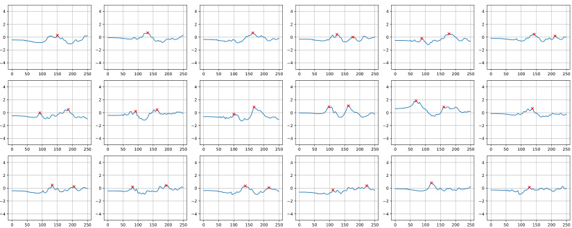
🔼 This figure presents an analysis of the Vibrating Plates dataset. Subfigure (a) displays two example plate geometries alongside their respective frequency response curves. Red crosses highlight the detected resonance peaks in the responses. Subfigure (b) shows the mean (average) plate design and its corresponding average frequency response across the entire dataset. Subfigure (c) illustrates the distribution of the number of resonance peaks observed across different dataset configurations. Finally, subfigure (d) shows the distribution of the peaks across the range of frequencies studied in the dataset.
read the caption
Figure 3: Dataset analysis. (a) shows two discretized plate geometries with their corresponding frequency response, the red crosses mark the detected peaks. (b) shows the mean plate design and frequency response. (c) shows number of peaks in different dataset settings. (d) shows the distribution of the peaks over the frequencies.

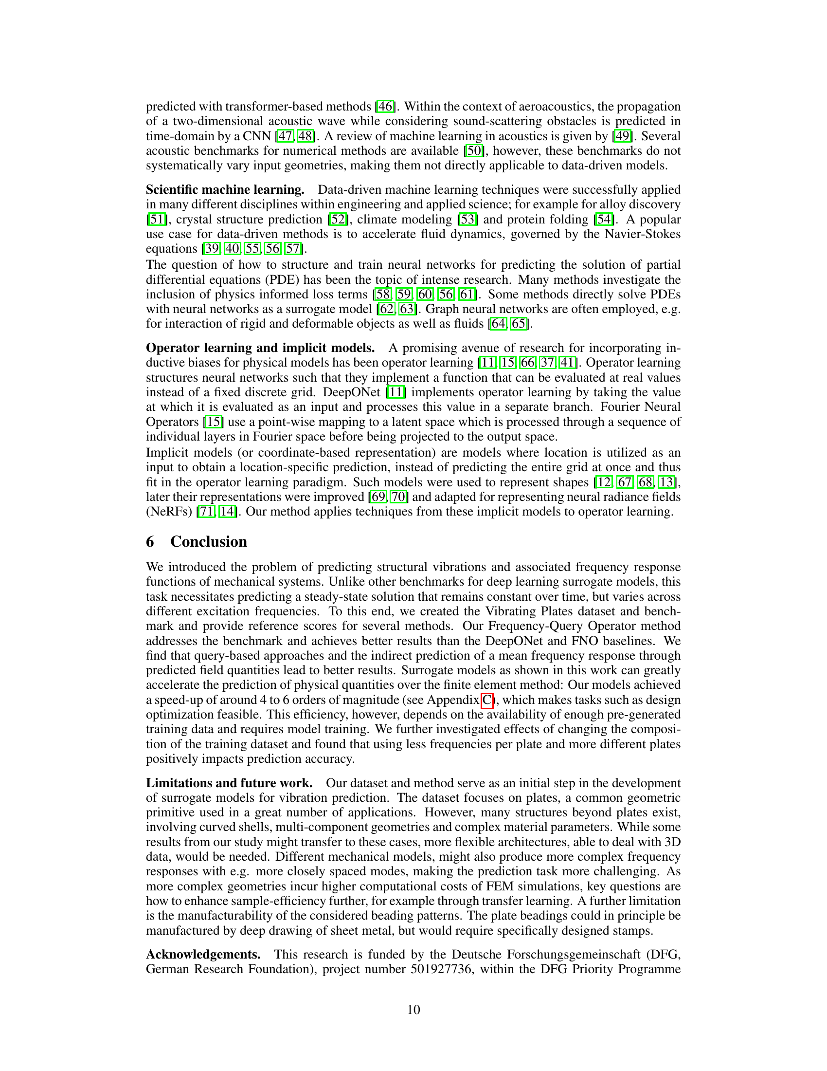
🔼 This figure illustrates the finite element method (FEM) used to simulate the vibrational behavior of plates. It shows the process of computing the velocity field at a specific excitation frequency. The process begins with a discretized plate geometry (finite element mesh) subjected to a harmonic point excitation at a given frequency. Numerical integration, system assembling, and solving a linear system of equations are then performed to obtain a field solution, represented as velocity maps at the queried frequency. These maps show the vibration pattern at that particular frequency, which is a key output of the model and a crucial part of the dataset.
read the caption
Figure 2: Process of the finite element solution in frequency domain in order to compute the velocity field at each frequency query.

🔼 The figure shows the architecture of the Frequency-Query Operator (FQO) model. The FQO model takes as input the mesh geometry of a plate and scalar properties. A geometry encoder processes this information and outputs a feature volume. This feature volume and a frequency query are then passed to a query decoder, which can either directly predict a frequency response or predict a velocity field which is then spatially aggregated to produce the frequency response. This architecture utilizes a query-based approach to handle variability in vibration characteristics across different instances.
read the caption
Figure 4: Frequency-Query Operator method. The geometry encoder takes the mesh geometry and the scalar properties as input. The resulting feature volume along with a frequency query is passed to the query decoder, that either predicts a velocity field or directly a frequency response. The velocity field is aggregated to arrive at the frequency response at the query frequency f.

🔼 This figure presents results from the FQO-UNet model. It demonstrates the velocity field predictions at a single frequency for a given plate geometry and compares them to ground truth. Furthermore, it illustrates the impact of dataset size and the number of frequencies per plate on model performance using mean squared error (MSE) as a metric. The analysis shows that reducing the number of samples or the number of frequencies per plate, while maintaining a fixed computational budget, can still yield reasonable results.
read the caption
Figure 5: Results. (b) to (d) show the velocity field at one frequency and prediction for the plate geometry in (a) from FQO-UNet. (e) shows the test MSE for training two methods with reduced numbers of samples from V-5000. (f) shows effects of different data generation strategies. The blue line is an isoconture for a fixed compute budget of 150,000 data points, with varying number of frequencies per plate geometry. The green star represents using a larger dataset at 15 frequencies per plate (half of V-5000). The red cross represents a model trained on V-5000. Training with fewer frequencies per plate is more efficient.

🔼 This figure shows the results of design optimization using a diffusion model guided by gradient information from the FQO-UNet. The leftmost panel displays an example of a generated beading pattern with reduced vibrations between 100Hz and 200Hz. The middle-left panel shows the best performing plate from the original V-5000 dataset for comparison. The middle-right panel presents a comparison of frequency responses. The rightmost panel shows frequency responses from 16 generated plates, demonstrating the model’s ability to generate diverse plate geometries with reduced vibrations in the target range.
read the caption
Figure 6: Design optimization. Exemplary generation result with lowest mean response between 100 Hz and 200 Hz out of 32 generations (left, mean response below). Plate with lowest response out of all 5000 training examples from V-5000 (middle left). Comparison of responses from left plates (middle right). Responses from 16 generated plates (right).
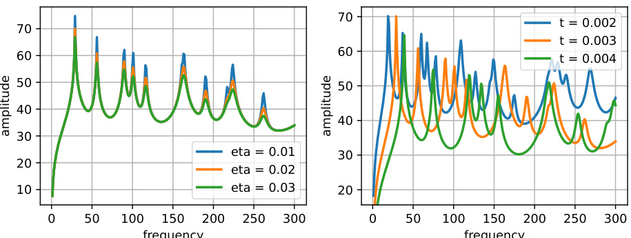
🔼 This figure shows the effect of varying the thickness and damping loss factor on the frequency response of a plate. The left plot demonstrates that increasing the damping loss factor (eta) reduces the amplitude of the resonance peaks without significantly shifting their frequencies. The right plot illustrates that increasing the plate thickness (t) increases the overall stiffness, resulting in a shift of the resonance peaks towards higher frequencies and a change in their amplitude.
read the caption
Figure 7: One-at-a-time parameter variation of the thickness parameter and the damping loss factor. Increasing the damping reduces the amplitudes at the resonance peaks. Increasing the plate thickness increases the stiffness of the plate and thus shifts the resonance peaks towards higher frequencies

🔼 This figure presents a detailed analysis of the Vibrating Plates dataset. Subfigure (a) illustrates the frequency response for two example plate geometries, highlighting the detected peaks. Subfigure (b) shows the average plate design and its corresponding frequency response. Subfigure (c) compares the number of peaks across different dataset configurations. Lastly, subfigure (d) displays the distribution of these peaks across the entire frequency range.
read the caption
Figure 3: Dataset analysis. (a) shows two discretized plate geometries with their corresponding frequency response, the red crosses mark the detected peaks. (b) shows the mean plate design and frequency response. (c) shows number of peaks in different dataset settings. (d) shows the distribution of the peaks over the frequencies.
🔼 This figure presents three examples of velocity field predictions from the V-5000 dataset, focusing on the frequencies corresponding to the three most prominent peaks in each example’s frequency response. The plots show both the ground truth (actual) velocity field and the model’s prediction for each frequency. The scaling applied to the plots normalizes the maximum velocity values to 1, highlighting the relative differences between the actual and predicted velocity field magnitudes.
read the caption
Figure 11: V-5000 example predictions. The velocity fields at the three peaks with the highest amplitude are shown. The plots are scaled with respect to the maximum velocity in the prediction and reference velocity field to make the differences in magnitude visible.

🔼 This figure presents an analysis of the Vibrating Plates dataset. Subfigure (a) illustrates two example plate geometries and their corresponding frequency response functions, highlighting detected peaks. (b) displays the mean plate design and its average frequency response function. (c) shows the number of peaks found across different dataset configurations and (d) visualizes the distribution of these peak counts across the frequency range.
read the caption
Figure 3: Dataset analysis. (a) shows two discretized plate geometries with their corresponding frequency response, the red crosses mark the detected peaks. (b) shows the mean plate design and frequency response. (c) shows number of peaks in different dataset settings. (d) shows the distribution of the peaks over the frequencies.
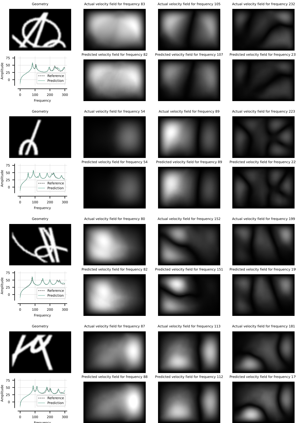
🔼 This figure presents example predictions from the V-5000 dataset. For each of the four example geometries, the actual and predicted velocity fields at the three frequencies with the highest amplitude are shown. The plots are scaled to highlight the differences in magnitude between actual and predicted velocity fields.
read the caption
Figure 11: V-5000 example predictions. The velocity fields at the three peaks with the highest amplitude are shown. The plots are scaled with respect to the maximum velocity in the prediction and reference velocity field to make the differences in magnitude visible.

🔼 This figure shows the results of the experiments performed. Subfigures (b) to (d) illustrate the velocity field predictions for a plate geometry using the FQO-UNet model, compared against the ground truth. Subfigure (e) displays the test MSE for two different models trained with varying amounts of data from the V-5000 dataset. Subfigure (f) compares the test MSE results obtained using three different data generation strategies with varying computational budgets and numbers of frequencies per geometry.
read the caption
Figure 5: Results. (b) to (d) show the velocity field at one frequency and prediction for the plate geometry in (a) from FQO-UNet. (e) shows the test MSE for training two methods with reduced numbers of samples from V-5000. (f) shows effects of different data generation strategies. The blue line is an isoconture for a fixed compute budget of 150,000 data points, with varying number of frequencies per plate geometry. The green star represents using a larger dataset at 15 frequencies per plate (half of V-5000). The red cross represents a model trained on V-5000. Training with fewer frequencies per plate is more efficient.
More on tables

🔼 This table presents the performance of various methods for predicting the frequency response of vibrating plates. It compares baseline methods (k-NN, RN18 + FNO, DeepONet, FNO (velocity field), Grid-RN18) against the proposed Frequency-Query Operator (FQO) using ResNet18 (FQO-RN18), Vision Transformer (FQO-ViT), and U-Net (FQO-UNet) architectures. The evaluation metrics include Mean Squared Error (MSE), Earth Mover’s Distance (EEMD), Peak Frequency Error (EPEAKS), and Peak Frequency Shift (EF). The VF and FQ columns indicate whether the method used velocity field prediction (Q3) and frequency queries (Q1), respectively. The results show that the proposed FQO methods significantly outperform the baseline methods.
read the caption
Table 1: Test results for frequency response prediction. Column VF indicates if F is indirectly predicted through the velocity field (Q3), column FQ indicates if frequency queries (Q1) are used. Q1 to Q3 refer to the model components described in Section 3.

🔼 This table presents the results of training a Frequency-Query Operator UNet model on two different datasets (V-5000 and G-5000), and then evaluating its performance on the G-5000 test dataset. The results are reported in terms of four evaluation metrics: Earth Mover’s Distance (EEMD), Mean Squared Error (MSE), Peak Frequency Error (EPEAKS), and Peak Frequency Shift (EF). The table shows that training the model on a combined dataset of V-5000 and G-5000 leads to improved performance compared to training solely on the G-5000 dataset, demonstrating the benefit of transfer learning in the context of the research.
read the caption
Table 3: A FQO-UNet is trained in parallel on batches from V-5000 and G-5000 and evaluated on the G-5000 test set. Performance increases in all metrics.

🔼 This table presents the configurations used in generating the V-5000 and G-5000 datasets. It shows how the plate geometries and material properties were varied to create the different samples. The ‘setting’ column refers to whether fixed (V-5000) or varying (G-5000) parameters were used. ‘Prop.’ specifies if material properties were fixed or varied. The ’lines’ and ’ellipses’ columns represent the number of lines and ellipses used in the beading patterns. ‘Width’ indicates the range of widths (in mm) of these beading features. Finally, ‘Train’ and ‘Test’ give the number of samples used for training and testing in each setting.
read the caption
Table 4: Dataset settings. Width is the width of lines and ellipses in mm. Properties. (prop.) involves plate size, thickness, material, boundary and loading properties.

🔼 This table presents the results of frequency response prediction using various methods. It compares the performance of different models in terms of Mean Squared Error (MSE), Earth Mover’s Distance (EEMD), Peak Frequency Error (EPEAKS), and the average distance between peaks (EF) on two datasets, V-5000 and G-5000. The table also indicates whether each model uses frequency queries (FQ) and/or predicts the velocity field (VF) before computing the frequency response.
read the caption
Table 1: Test results for frequency response prediction. Column VF indicates if F is indirectly predicted through the velocity field (Q3), column FQ indicates if frequency queries (Q1) are used. Q1 to Q3 refer to the model components described in Section 3.

🔼 This table presents the performance of various methods for predicting the frequency response of vibrating plates. It compares different model architectures (including baselines and the proposed Frequency-Query Operator), showing mean squared error (MSE), Earth Mover’s Distance (EEMD), and Peak Frequency Error (EPEAKS) metrics. The VF column indicates whether the model indirectly predicts the frequency response via the velocity field, and the FQ column indicates whether frequency queries were used as input. Lower values for the error metrics indicate better performance.
read the caption
Table 1: Test results for frequency response prediction. Column VF indicates if F is indirectly predicted through the velocity field (Q3), column FQ indicates if frequency queries (Q1) are used. Q1 to Q3 refer to the model components described in Section 3.

🔼 This table presents the performance of different methods for predicting the frequency response of vibrating plates. It compares various deep learning approaches (FQO-RN18, FQO-ViT, FQO-UNet, and baselines like DeepONet and FNO) on two datasets (V-5000 and G-5000), evaluating their Mean Squared Error (MSE), Earth Mover’s Distance (EEMD), Peak Frequency Error (EPEAKS), and the average frequency error (EF). The ‘VF’ column indicates whether the model predicts the velocity field and then calculates the frequency response, and ‘FQ’ shows if the model incorporates frequency queries. Lower values for MSE, EEMD, EPEAKS, and EF indicate better performance.
read the caption
Table 1: Test results for frequency response prediction. Column VF indicates if F is indirectly predicted through the velocity field (Q3), column FQ indicates if frequency queries (Q1) are used. Q1 to Q3 refer to the model components described in Section 3.

🔼 This table presents the results of frequency response prediction using various methods. The table compares different methods (baselines and the proposed FQO method) across two datasets (V-5000 and G-5000). The evaluation metrics include Mean Squared Error (MSE), Earth Mover Distance (EEMD), Peak Frequency Error (EPEAKS), and the average frequency error (EF). The columns ‘VF’ and ‘FQ’ indicate whether the velocity field was used for prediction and whether frequency queries were employed, respectively.
read the caption
Table 1: Test results for frequency response prediction. Column VF indicates if F is indirectly predicted through the velocity field (Q3), column FQ indicates if frequency queries (Q1) are used. Q1 to Q3 refer to the model components described in Section 3.

🔼 This table presents the quantitative results of various methods used for frequency response prediction on the V-5000 and G-5000 datasets. The methods are compared using four metrics: Mean Squared Error (MSE), Earth Mover’s Distance (EEMD), Peak Frequency Error (EPEAKS), and the average peak frequency shift (EF). The table also indicates whether each method used a velocity field (VF) and frequency query (FQ) approach, corresponding to questions Q1-Q3 in the paper, allowing for analysis of the impact of these architectural decisions on prediction accuracy.
read the caption
Table 1: Test results for frequency response prediction. Column VF indicates if F is indirectly predicted through the velocity field (Q3), column FQ indicates if frequency queries (Q1) are used. Q1 to Q3 refer to the model components described in Section 3.

🔼 This table presents the performance of various methods for predicting the frequency response of vibrating plates. It compares different model architectures, including baselines and the proposed Frequency-Query Operator (FQO), across two datasets (V-5000 and G-5000). The metrics used to evaluate performance are Mean Squared Error (MSE), Earth Mover’s Distance (EEMD), Peak Frequency Error (EPEAKS), and Peak Frequency Shift (EF). The VF and FQ columns indicate whether the model uses velocity field prediction and frequency queries, respectively, as described in Section 3 of the paper.
read the caption
Table 1: Test results for frequency response prediction. Column VF indicates if F is indirectly predicted through the velocity field (Q3), column FQ indicates if frequency queries (Q1) are used. Q1 to Q3 refer to the model components described in Section 3.

🔼 This table presents the test results of various methods for frequency response prediction. It compares different model architectures (including baselines) on two datasets (V-5000 and G-5000). The metrics used to evaluate the models are Mean Squared Error (MSE), Earth Mover Distance (EEMD), Peak Frequency Error (EPEAKS), and the average frequency shift (EF). The ‘VF’ column indicates whether the model indirectly predicts the frequency response through the velocity field, and the ‘FQ’ column indicates whether the model uses frequency queries as input.
read the caption
Table 1: Test results for frequency response prediction. Column VF indicates if F is indirectly predicted through the velocity field (Q3), column FQ indicates if frequency queries (Q1) are used. Q1 to Q3 refer to the model components described in Section 3.

🔼 This table presents the performance of various models on the task of frequency response prediction. It compares different model architectures, including baselines (k-NN, RN18 + FNO, DeepONet, etc.) and the proposed Frequency-Query Operator (FQO) method in variations (FQO-RN18, FQO-ViT, FQO-UNet). Evaluation metrics used are Mean Squared Error (MSE), Earth Mover’s Distance (EEMD), Peak Frequency Error (EPEAKS), and average Peak Frequency shift (EF). The ‘VF’ column indicates whether the model uses velocity field prediction and ‘FQ’ shows whether it uses frequency query. The table shows results for two different dataset settings (V-5000 and G-5000) which vary in the number of parameters used to describe the plates.
read the caption
Table 1: Test results for frequency response prediction. Column VF indicates if F is indirectly predicted through the velocity field (Q3), column FQ indicates if frequency queries (Q1) are used. Q1 to Q3 refer to the model components described in Section 3.
Full paper#


