↗ OpenReview ↗ NeurIPS Homepage ↗ Chat
TL;DR#
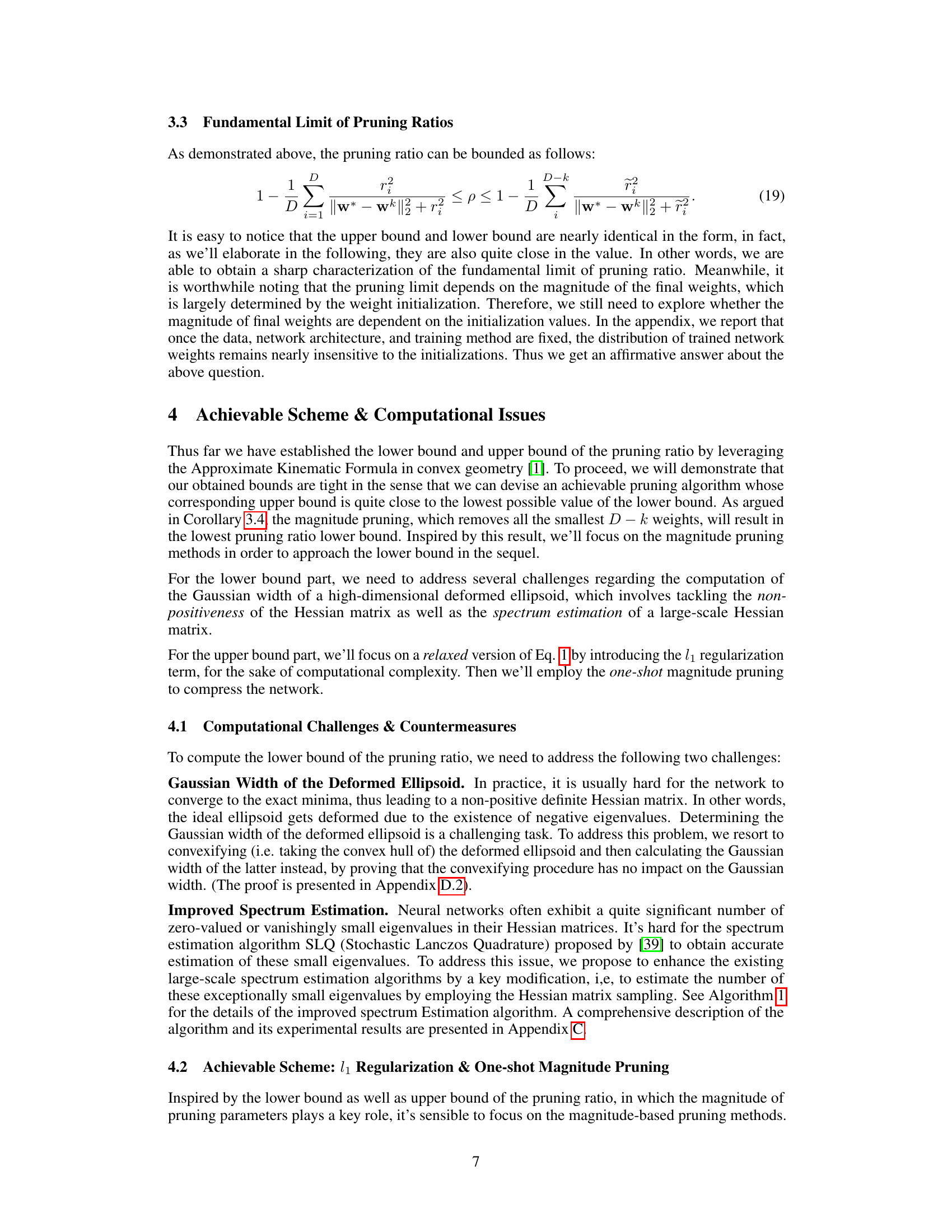
Deep neural networks (DNNs), while powerful, are computationally expensive due to their massive size. Network pruning, a technique to remove less important connections, aims to address this. However, a crucial question remained unanswered: what’s the maximum level of pruning possible without significantly harming performance? This research tackles this using convex geometry to understand the loss landscape, essentially determining how much a DNN can be pruned before the sublevel set (all weights within a certain loss range) stops intersecting with the set of sparse networks (networks with the desired pruning). This analysis reveals that pruning limits depend on two key factors: the magnitude of weights and the network sharpness (related to the curvature of the loss function).
The researchers provide mathematical proofs and formulas to accurately predict this pruning limit. They demonstrate a powerful countermeasure for computational challenges in calculating the pruning limit, mainly regarding the spectral estimation of large, non-positive definite Hessian matrices. Experiments confirm that their theoretical predictions closely align with practical results. They also provide intuitive explanations of several widely used pruning heuristics, suggesting why certain pruning strategies work better than others.
Key Takeaways#
Why does it matter?#
This paper is crucial because it establishes the fundamental limits of deep neural network pruning, a widely used technique for improving efficiency. By providing both upper and lower bounds for the pruning ratio, it provides a theoretical framework for guiding future pruning algorithm development and informs better design choices. This has a significant impact on resource-constrained applications where efficiency is paramount.
Visual Insights#

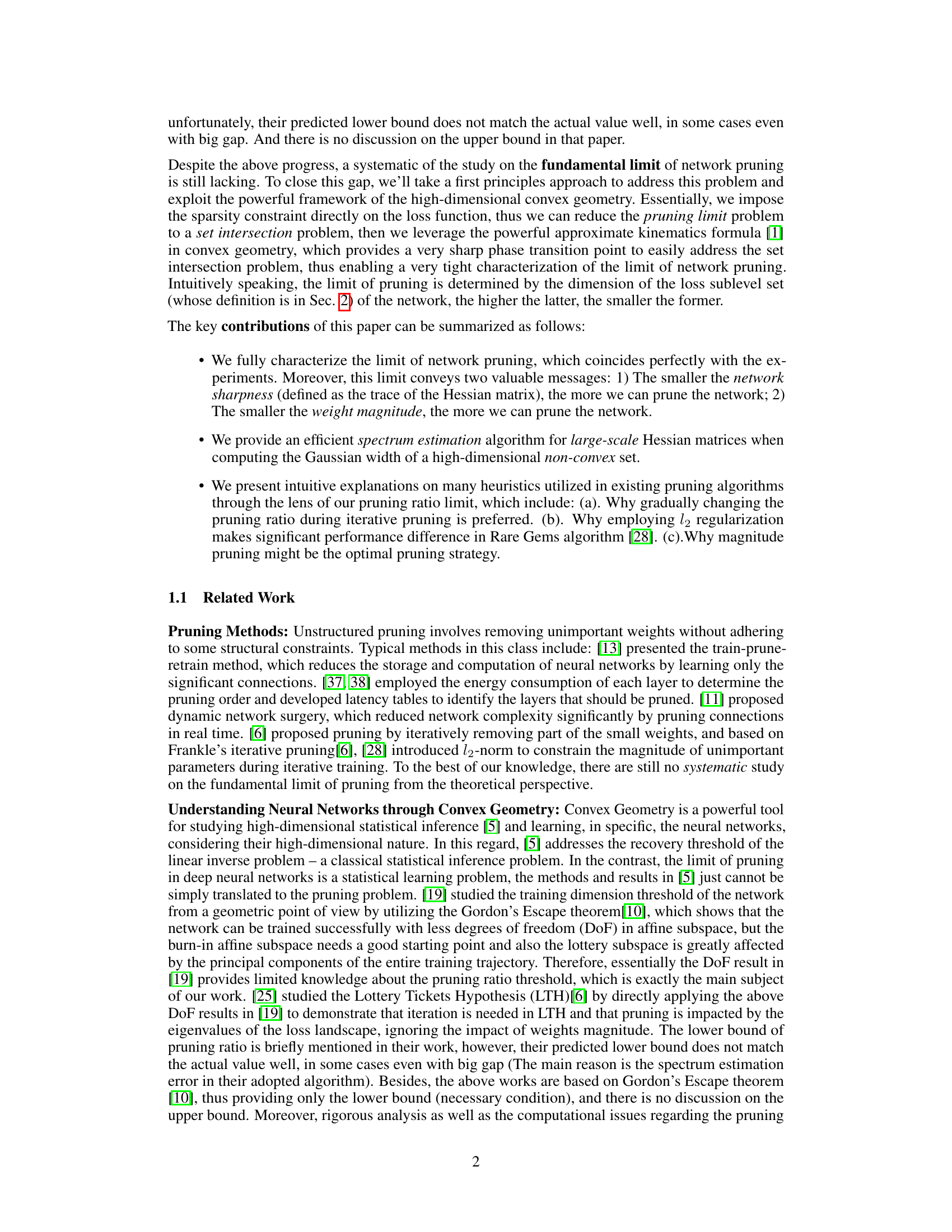
This figure illustrates three key concepts from convex geometry that are central to the paper’s theoretical framework. Panel (a) shows a convex cone, which is a set of vectors that are closed under positive scalar multiplication. Panel (b) demonstrates how the statistical dimension of a cone affects its size; a larger statistical dimension corresponds to a larger cone. Finally, panel (c) shows the effect of the distance between a subspace and a convex set on their intersection probability; the closer they are, the higher the probability of intersection. These concepts are used to analyze the fundamental limits of network pruning by relating it to the problem of set intersection in high-dimensional space.

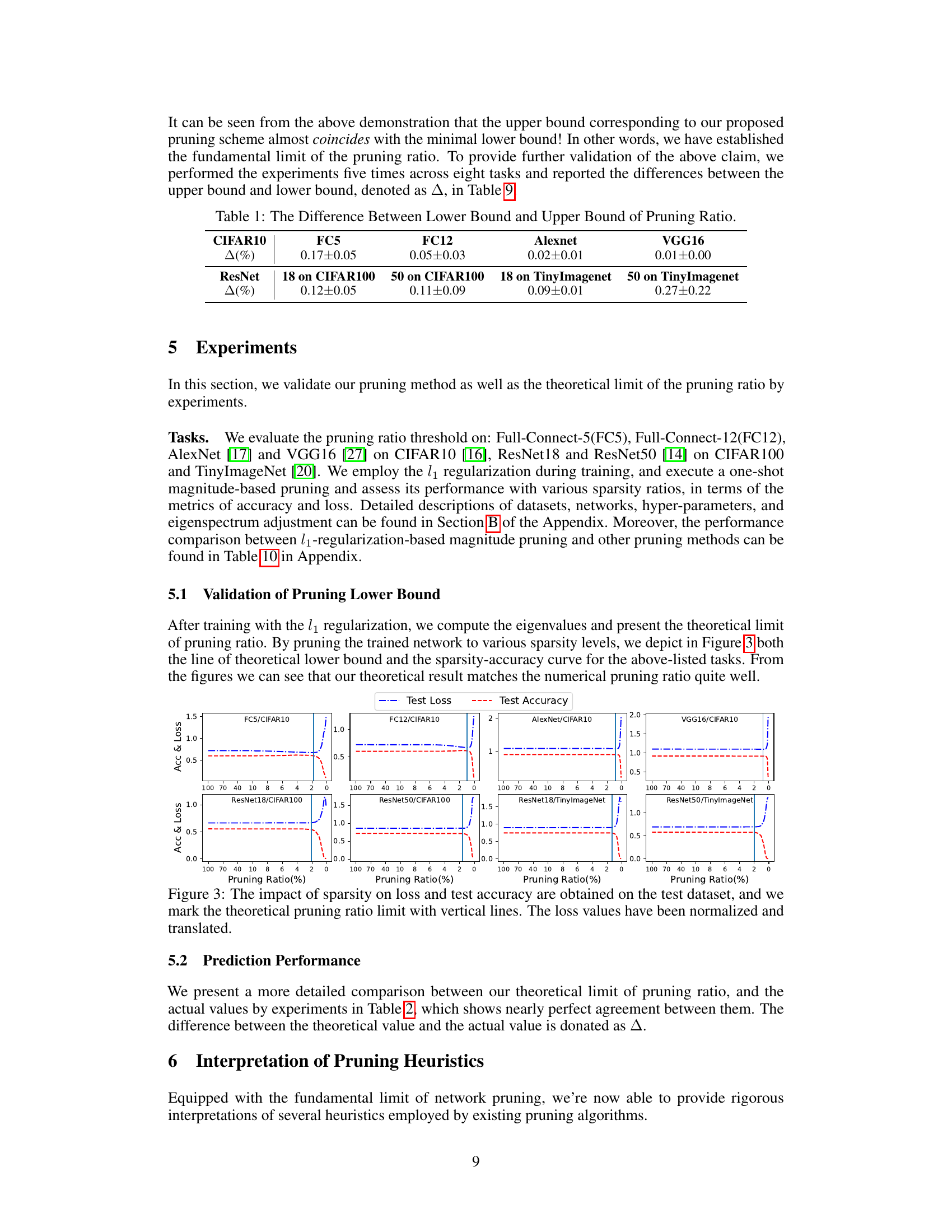
This table presents the difference between the theoretically calculated lower bound and upper bound of the pruning ratio for various network architectures and datasets. The smaller the difference (Δ), the tighter the bounds and the more accurate the theoretical prediction of the pruning limit.
In-depth insights#
Pruning Limits#
The concept of “Pruning Limits” in deep neural network research explores the fundamental constraints on how much a network can be simplified (pruned) while maintaining acceptable performance. Understanding these limits is crucial for efficient model deployment, as it guides the development of effective pruning algorithms and prevents excessive simplification, which can harm performance. Research in this area often focuses on identifying key factors influencing these limits, such as network architecture, training data characteristics, and the pruning methodology itself. Determining a precise theoretical pruning limit remains a challenge, with studies often relying on approximations and empirical observations. The pursuit of optimal pruning strategies is an ongoing process, with future research likely to refine our understanding of these limitations and pave the way for more efficient and effective network pruning techniques. Finding the balance between sparsity and accuracy is a key focus, as is understanding the underlying mathematical and statistical properties that govern the relationship between network structure and predictive capability.
Convex Geometry#
Convex geometry provides a powerful framework for analyzing high-dimensional spaces, particularly relevant to machine learning and deep neural networks. Its core concepts, such as convex sets, cones, and hulls, offer a geometric lens through which to study complex optimization problems. By characterizing properties of these shapes—like their widths or dimensions—we gain valuable insights into the behavior of algorithms. In the context of neural networks, convex geometry helps to analyze loss landscapes, understand the impact of model size and sparsity, and characterize the existence and properties of optimal solutions. The statistical dimension, a key concept borrowed from convex geometry, provides a quantitative measure of the complexity of a problem, directly influencing the feasibility of various optimization techniques, including pruning strategies. Therefore, understanding and leveraging tools from convex geometry is crucial for both theoretical analysis and improved algorithm design in the field of deep learning.
Hessian Spectrum#
Analyzing the Hessian spectrum in the context of deep learning reveals crucial insights into the loss landscape’s geometry and its impact on network training and pruning. The eigenvalues of the Hessian matrix directly reflect the curvature of the loss function around a critical point, revealing whether the landscape is sharply peaked (high curvature, large eigenvalues) or relatively flat (low curvature, small eigenvalues). In network pruning, a flatter landscape is highly desirable as it implies greater robustness to weight removal, indicating that the model’s performance is less sensitive to parameter changes. The spectrum’s distribution provides key information about the model’s generalization capability and training dynamics. A heavily skewed spectrum may suggest overparameterization, while a more uniform distribution might indicate a better-conditioned optimization problem. Efficient and accurate computation of the Hessian spectrum, however, presents significant challenges, especially for large-scale networks, because it is computationally expensive and the Hessian might be ill-conditioned or not positive semi-definite. Effective techniques like stochastic Lanczos quadrature are crucial for approximating the spectrum and addressing these computational bottlenecks. Future research can focus on developing faster and more robust methods for Hessian spectrum estimation as well as exploring further connections between the Hessian spectrum and other key properties of deep learning models such as generalization error and robustness.
L1 Regularization#
L1 regularization, also known as Lasso regularization, is a powerful technique used in machine learning to constrain model complexity and prevent overfitting. It achieves this by adding a penalty term to the loss function that is proportional to the sum of the absolute values of the model’s weights. This penalty encourages sparsity, meaning that many weights will be driven to zero during training. This sparsity has several benefits: it can improve the model’s generalization performance on unseen data, make the model more interpretable by selecting only the most important features, and reduce the computational cost of prediction. The choice between L1 and L2 regularization often depends on the specific problem and desired properties. L1 regularization is particularly useful when feature selection is important, as it tends to produce sparse models with many zero-weighted features. In contrast, L2 regularization (Ridge regression) shrinks weights towards zero, but rarely results in them being exactly zero. The strength of the L1 penalty is controlled by a hyperparameter (often called λ or α), which requires careful tuning via techniques like cross-validation to find the optimal balance between model complexity and performance. Choosing the right λ is crucial for effectiveness; too small and the penalty has little impact, too large and it leads to underfitting. The impact of L1 regularization can also vary depending on the dataset characteristics, the model architecture, and the optimization algorithm used.
Future Work#
Future research directions stemming from this work could explore several promising avenues. Extending the theoretical framework to encompass more complex network architectures beyond the fully-connected and convolutional models analyzed would significantly broaden the applicability of the fundamental pruning limits. Investigating the impact of different training methodologies and regularization techniques on these limits is crucial for practical implementation. The current work focuses on a single-shot pruning strategy; therefore, analyzing the theoretical limitations and opportunities presented by iterative pruning approaches deserves attention. Finally, developing computationally efficient algorithms to estimate the Hessian matrix spectrum for very large-scale networks remains a significant challenge that warrants further investigation. Addressing these questions will provide a more complete understanding of network pruning and pave the way for the development of more effective and efficient pruning strategies.
More visual insights#
More on figures

This figure provides a visual representation of key concepts in high-dimensional convex geometry used in the paper. Panel (a) and (b) illustrate how the size of a convex cone influences its statistical dimension, a measure of complexity. Panel (c) shows how the projection distance affects the size of a projected set and its probability of intersecting with a given subspace, relating to the feasibility of network pruning.

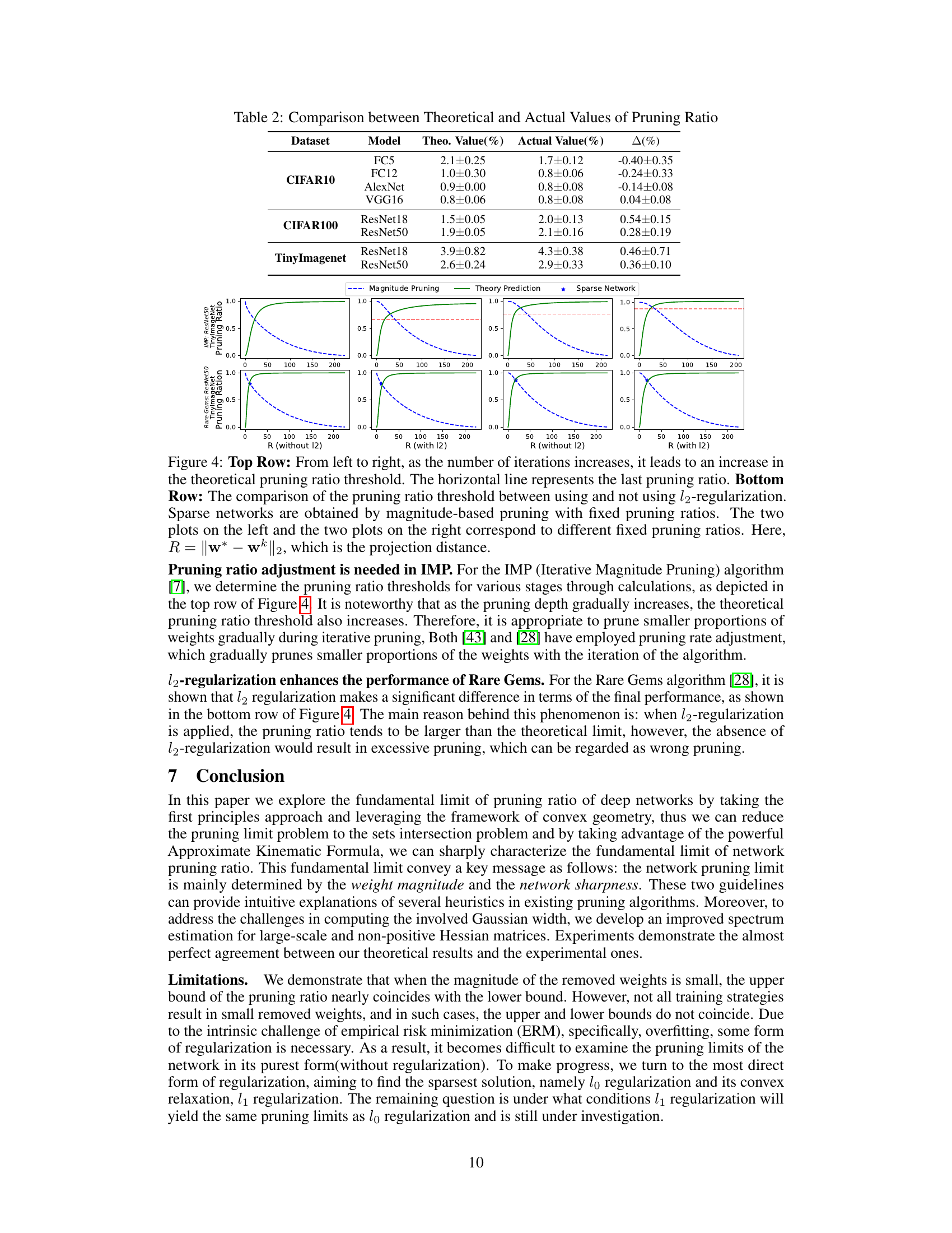
This figure shows the impact of different pruning ratios on the test loss and accuracy for various network architectures and datasets. Each subfigure represents a specific model (e.g., FC5, ResNet18) trained on a particular dataset (e.g., CIFAR10, CIFAR100). The x-axis represents the pruning ratio (percentage of weights removed), and the y-axis represents the test loss and accuracy. Vertical lines indicate the theoretical pruning ratio limit calculated by the authors’ method. The results demonstrate a close agreement between the theoretical limit and the experimental observations of loss and accuracy.

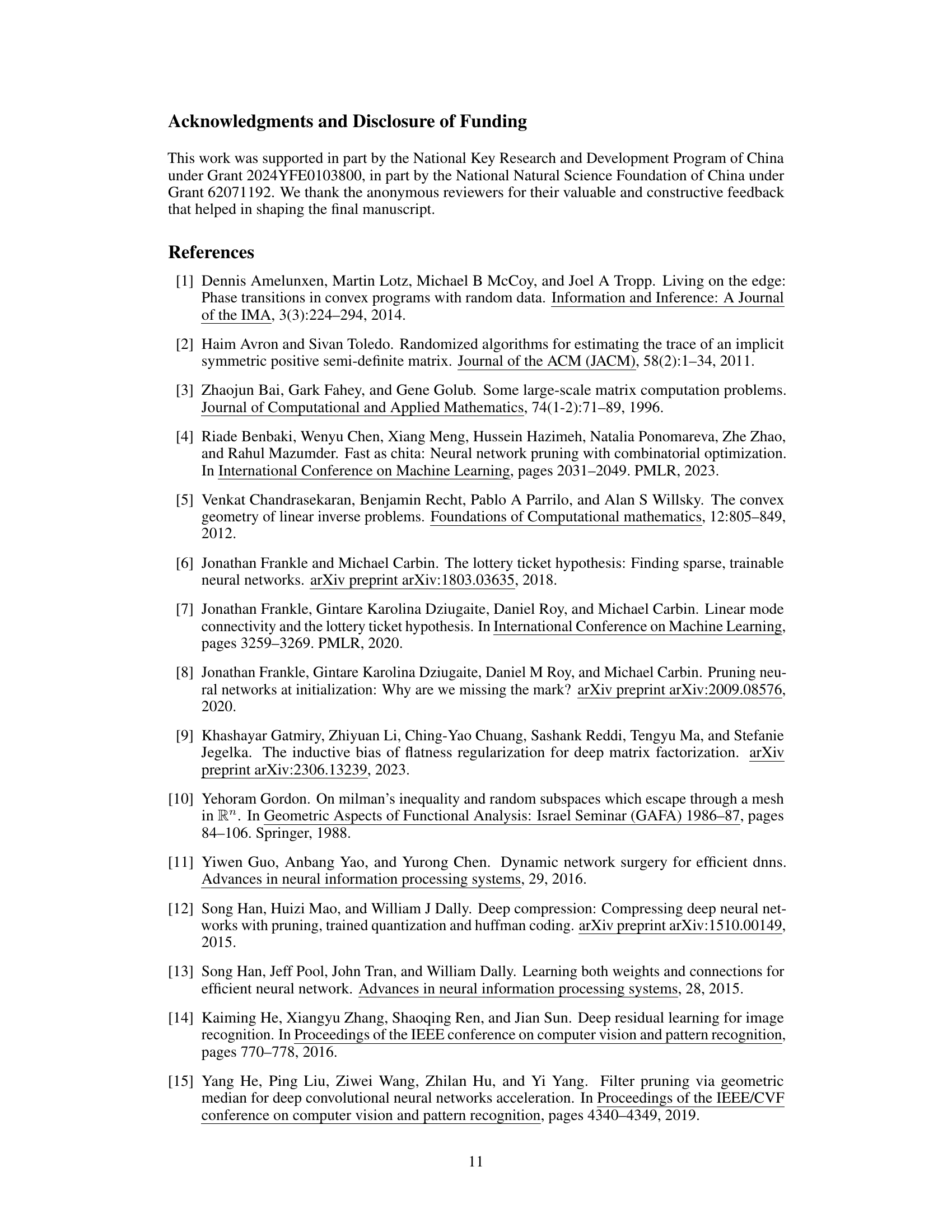
This figure visualizes the impact of iterative pruning and l2 regularization on the pruning ratio. The top row demonstrates how the theoretical pruning ratio threshold increases with more iterations, while the bottom row compares the threshold with and without l2 regularization. The plots show that iterative pruning gradually increases the pruning ratio, while l2 regularization enhances the performance of the Rare Gems algorithm by increasing the pruning threshold.

This figure shows a comparison of the theoretical pruning ratio predictions against the actual pruning ratios obtained using magnitude pruning for eight different model-dataset combinations. The top row shows results for smaller, fully connected networks (FC5, FC12) and convolutional networks (AlexNet, VGG16) trained on CIFAR-10. The bottom row displays results for larger ResNet models (ResNet18 and ResNet50) trained on CIFAR-100 and TinyImageNet datasets. For each task, the theoretical curve predicts the minimum pruning ratio that can be achieved without sacrificing performance. The actual pruning ratios (obtained by experiment) are plotted alongside these theoretical predictions to validate the theory.

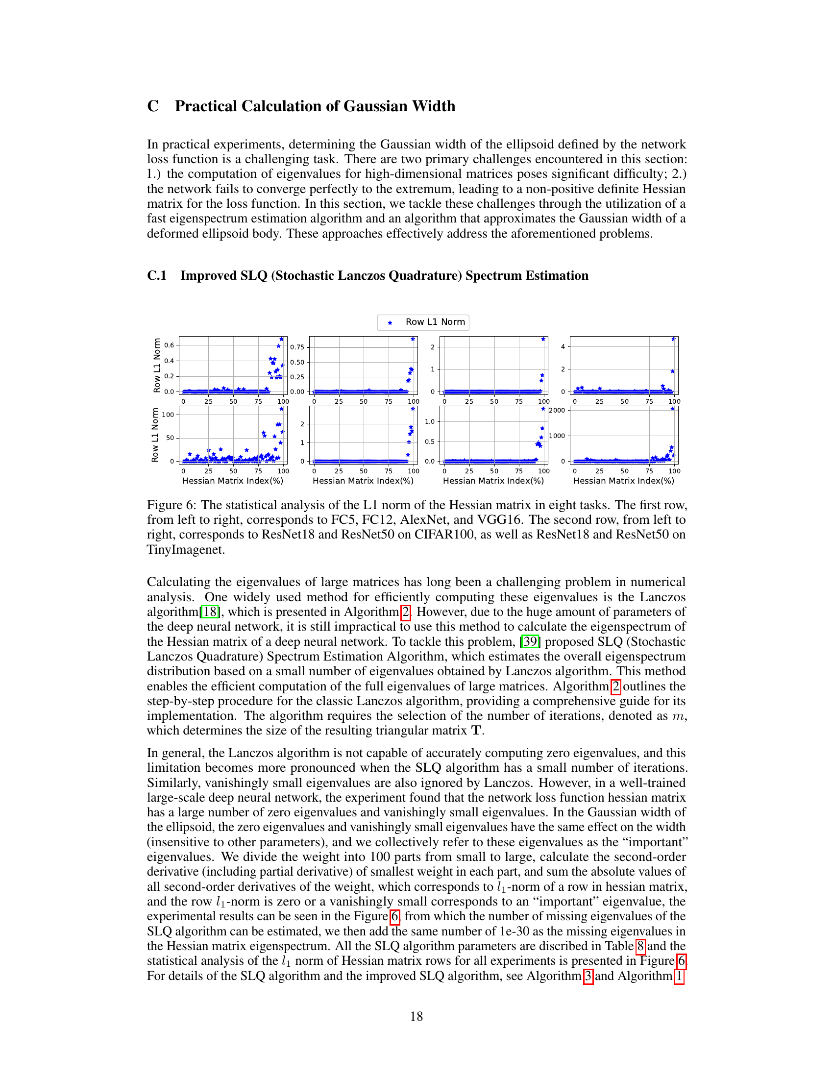
This figure shows the L1 norm of each row in the Hessian matrix for eight different network architectures trained on various datasets. The x-axis represents the percentage of rows in the Hessian matrix, and the y-axis represents the L1 norm of those rows. Each subplot displays the L1 norm distribution for a specific network and dataset combination, illustrating the heterogeneity in the Hessian matrix’s row-wise magnitudes. This analysis is important for understanding the network’s structure and the relative significance of different parameters. The concentration of low L1 norm values is especially notable.
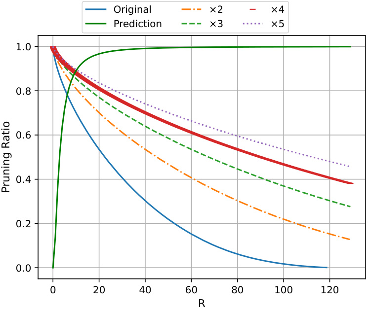
This figure displays the relationship between pruning ratio and the magnitude of weights. It shows how the pruning ratio changes as the magnitude of weights increases. The ‘Original’ curve represents the pruning ratio without any modifications to the weight magnitudes. The other curves (‘x2’, ‘x3’, ‘x4’, ‘x5’) show the predicted pruning ratios when the magnitude of weights is multiplied by 2, 3, 4, and 5 respectively. The green curve labeled ‘Prediction’ shows an approximation for the pruning ratio. The figure highlights that as the magnitude of weights increases, the achievable pruning ratio decreases.

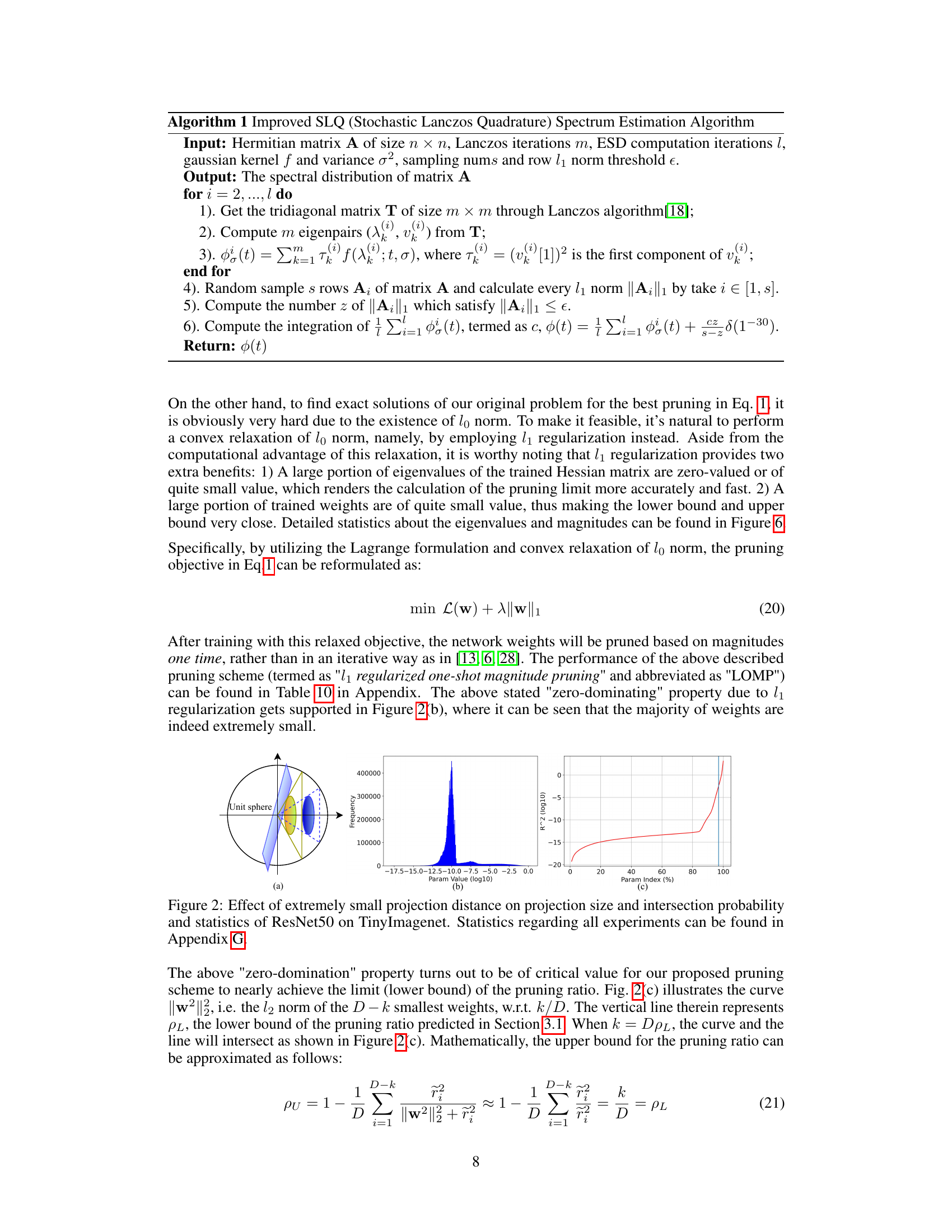
This figure shows the distribution of weights and the relationship between the pruning ratio and the magnitude of weights for eight different tasks. The top row shows the results for FC5, FC12, AlexNet, and VGG16 on CIFAR10. The bottom row shows the results for ResNet18 and ResNet50 on CIFAR100 and TinyImageNet. For each task, there are two plots. The left plot shows the distribution of the weights (in log scale), and the right plot shows the relationship between the pruning ratio and the magnitude of the weights. The red curve in the right plot represents the theoretical prediction for the pruning ratio based on the paper’s proposed model, and the blue curve represents the actual observed pruning ratio.
More on tables

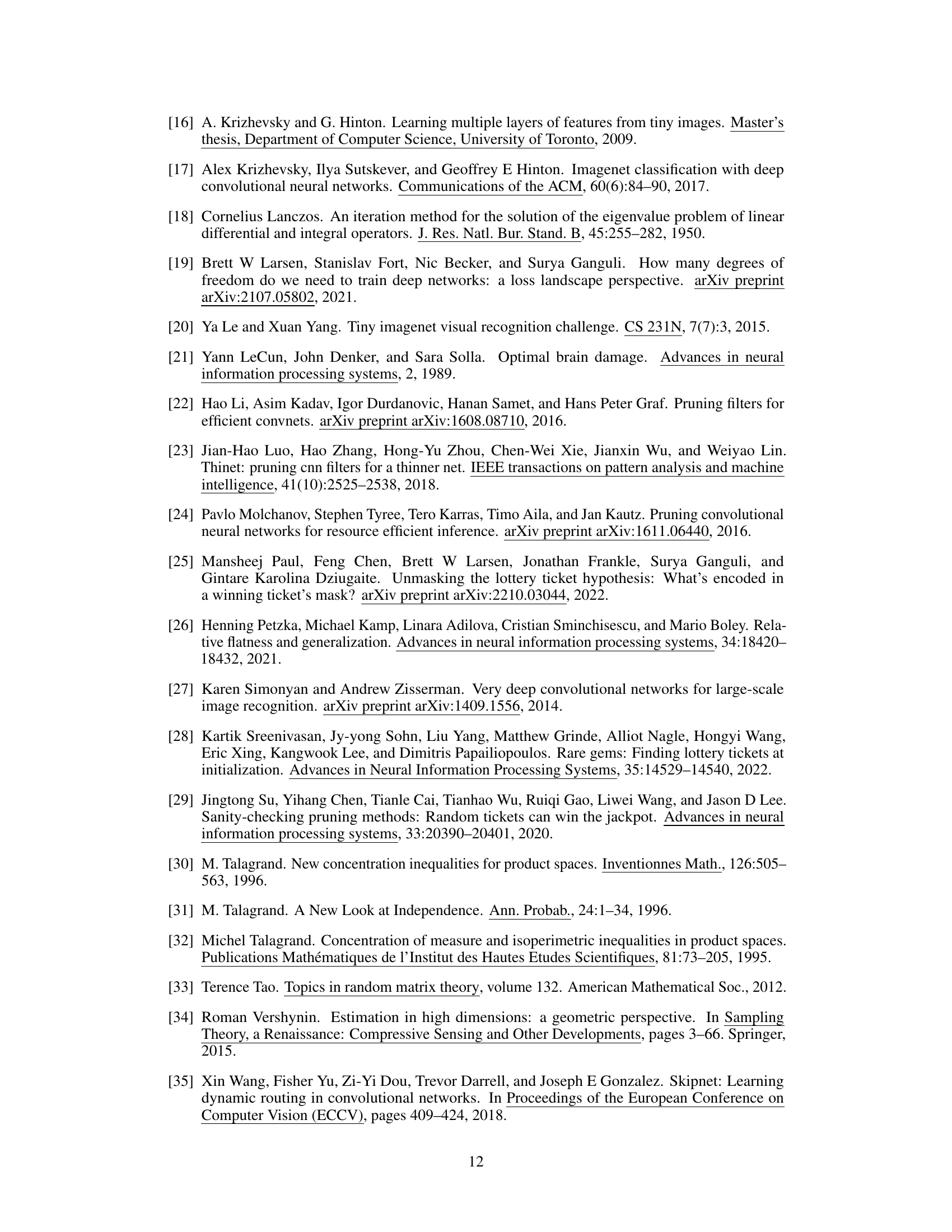
This table presents a comparison of the theoretical and actual pruning ratios obtained from experiments across various datasets and models. The ‘Theo. Value’ column shows the theoretically predicted pruning ratios based on the paper’s formulas, while the ‘Actual Value’ column displays the empirically observed pruning ratios. The difference between the theoretical and actual values, expressed as a percentage, is provided in the Δ column. This comparison helps validate the accuracy of the theoretical model proposed in the paper for predicting pruning ratios.

This table compares the performance of the proposed one-shot magnitude pruning algorithm (‘LOMP’) with four baseline algorithms: dense training and three other pruning algorithms (Rare Gems, Iterative Magnitude Pruning, and Smart-Ratio). The comparison is done across various datasets and models, considering the test accuracy achieved at different sparsity levels. The results showcase the superior performance of the proposed LOMP algorithm compared to the other methods.

This table compares the theoretical pruning ratios calculated using the formulas derived in the paper with the actual pruning ratios observed in experiments across various datasets and network architectures. The percentage difference between the theoretical and actual values is also provided to show the accuracy of the theoretical predictions.

This table presents a comparison of the performance of different pruning algorithms, including the proposed LOMP method and four baseline methods (dense weight training, Rare Gems, Iterative Magnitude Pruning, and Smart-Ratio). The performance is evaluated in terms of test accuracy at top-1, using different sparsity levels. The results show that the proposed LOMP algorithm outperforms the baseline methods across various datasets and network architectures.

This table presents a comparison of the performance of different pruning algorithms, including the proposed LOMP method and several baselines (dense training, Rare Gems, Iterative Magnitude Pruning, and Smart-Ratio). The performance is evaluated across different datasets and models in terms of accuracy at top-1 and sparsity. It demonstrates the superior performance of the proposed LOMP algorithm, particularly at higher sparsity levels.

This table lists the hyperparameters used for training different deep neural network models on various datasets. It shows the batch size, number of epochs, optimizer (Stochastic Gradient Descent), learning rate (LR), momentum, warm-up period, weight decay, use of cosine annealing learning rate schedule (CosineLR), and the lambda regularization parameter. Each row represents a unique model-dataset combination with its corresponding hyperparameter settings.

This table shows the hyperparameters used in the Stochastic Lanczos Quadrature (SLQ) algorithm for computing the Gaussian width. The hyperparameters include the number of runs, iterations, bins, and squared sigma for different models and datasets. These parameters are crucial for the accurate estimation of the Gaussian width, which is a key component in the paper’s theoretical analysis of the pruning ratio.

This table presents the total variation (TV) distance between the distributions of trained weights for different network architectures (FC5, FC12, AlexNet, VGG16, ResNet18, ResNet50) trained on various datasets (CIFAR10, CIFAR100, TinyImagenet). The TV distance measures the difference between the weight distributions obtained from multiple independent training runs. The smaller the distance, the more similar the weight distributions across training runs, suggesting the weight distribution is consistent and independent of the specific initialization. This table validates the robustness of the weight magnitude distribution regardless of initialization.

This table compares the performance of the proposed LOMP algorithm with several other pruning algorithms (RG, IMP, SR) across various datasets and models. It shows the dense accuracy, sparsity, and top-1 test accuracy for each method. LOMP consistently outperforms the other methods, especially at higher sparsity levels.
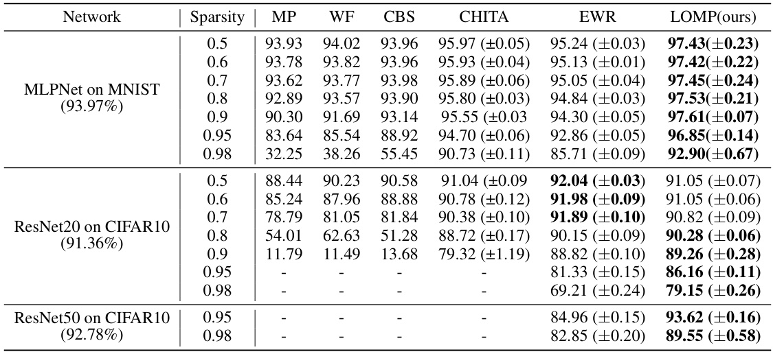
This table compares the pruning performance (model accuracy) of the proposed LOMP algorithm against other state-of-the-art pruning methods. The comparison is conducted on three different network architectures (MLPNet, ResNet20, and ResNet50) at various sparsity levels. The results demonstrate the superiority of LOMP, particularly at high sparsity levels.
Full paper#

