↗ OpenReview ↗ NeurIPS Homepage ↗ Chat
TL;DR#
Merging multiple neural networks can boost performance, but existing methods struggle with inconsistencies, especially when merging three or more models. These methods often create an accumulation of errors when combining the models, resulting in inferior performance compared to the original models. Pairwise model merging approaches fail to guarantee this cycle consistency.
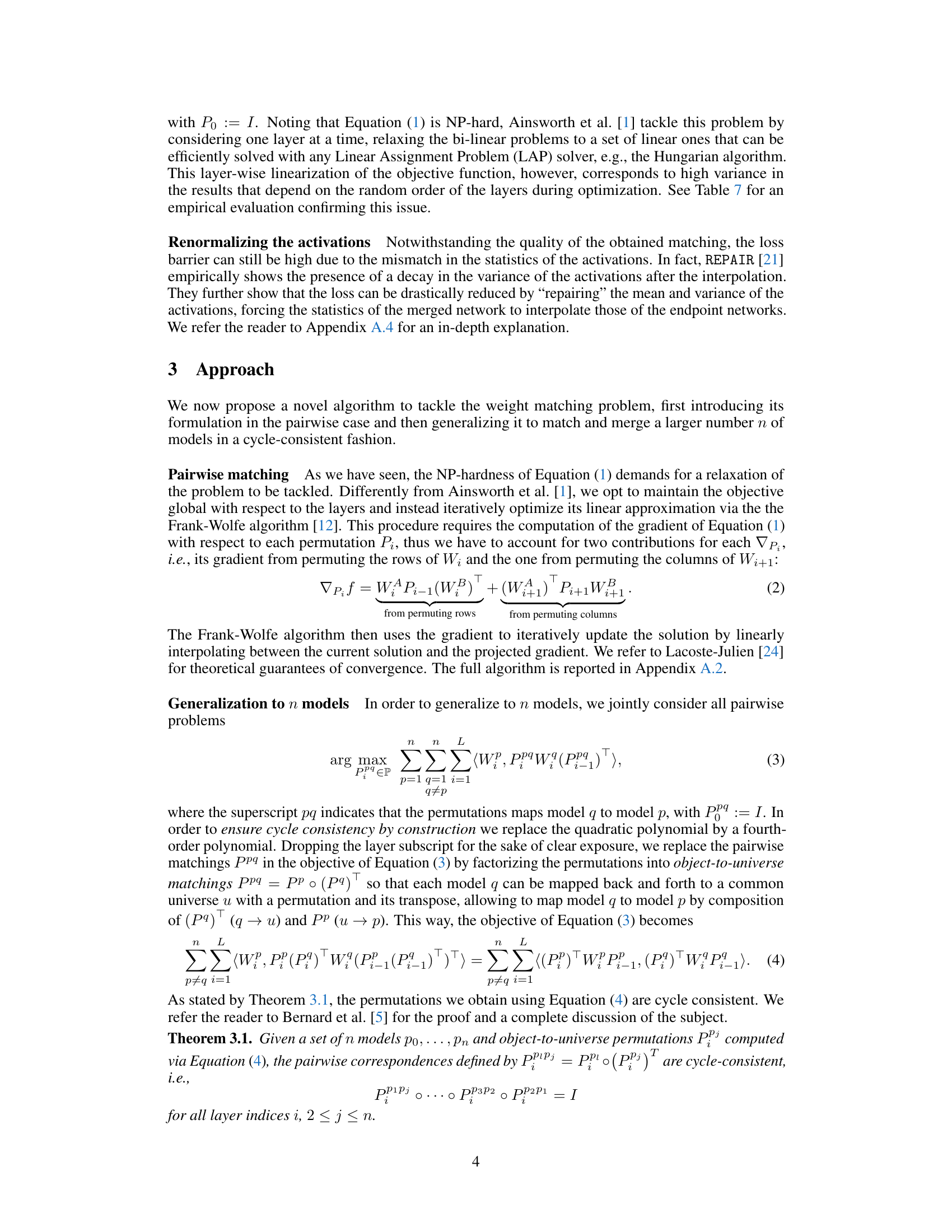
C2M³, the method proposed in this paper, directly addresses these issues. By mapping each network to a common ‘universe’ space, and enforcing cycle consistency among the mappings, C2M³ effectively merges multiple models. This data-free approach leverages the Frank-Wolfe algorithm for efficient optimization and incorporates activation renormalization to further improve the results. The method was extensively tested on various architectures and datasets, yielding better results than current state-of-the-art methods. The authors provide a publicly available codebase to foster reproducibility.
Key Takeaways#
Why does it matter?#
This paper is crucial for researchers in deep learning and neural network optimization. It addresses the significant challenge of merging multiple neural network models effectively, a problem with implications for improving model performance, efficiency, and robustness. The novel cycle-consistent merging method provides a significant advance over existing techniques and opens avenues for future research into efficient and robust model aggregation. Its emphasis on data-free methods and cycle consistency is particularly relevant in contexts where large datasets may not be available or computational resources are limited.
Visual Insights#
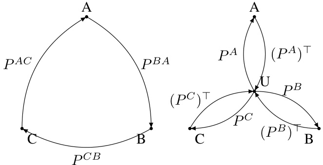
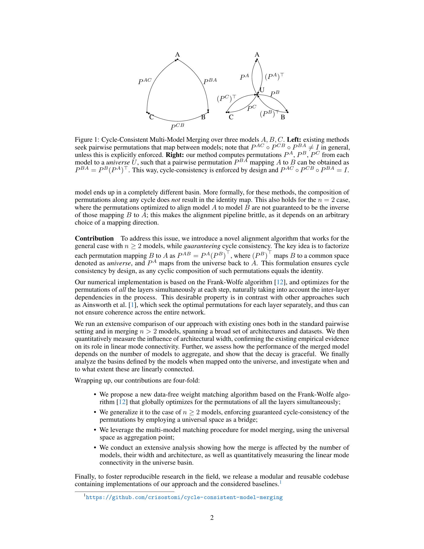
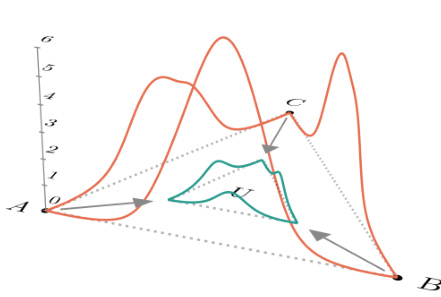
This figure illustrates the difference between existing pairwise model merging methods and the proposed cycle-consistent approach. The left panel shows that existing methods may not satisfy cycle consistency, i.e., the composition of pairwise mappings does not necessarily result in the identity transformation. In contrast, the right panel shows that the proposed approach introduces a universal space U, mapping each model A, B, and C to it. It enforces cycle consistency by design, as the composition of pairwise mappings through U always leads to the identity transformation.
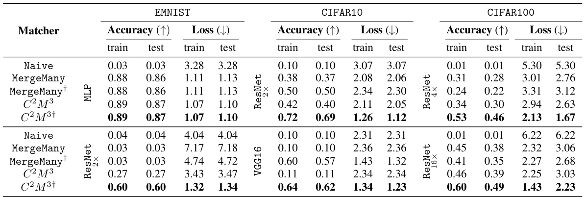
This table shows the accuracy and loss for different model merging methods. It compares a naive averaging method, MergeMany, and the proposed C2M³ approach, both with and without activation renormalization (REPAIR). Results are shown for different model architectures (MLP, ResNet, VGG16) and datasets (EMNIST, CIFAR10, CIFAR100). The best-performing method is highlighted in bold. The table demonstrates the superior performance of the C2M³ approach, especially when coupled with REPAIR.
In-depth insights#
Cycle-Consistent Merging#
Cycle-consistent merging in neural networks addresses the limitations of pairwise merging methods by enforcing consistency across multiple models. Existing pairwise methods often struggle with accumulating errors when merging more than two models, resulting in inconsistencies. This cycle-consistent approach factors each permutation mapping between models through a shared “universe” space, ensuring that the composition of any cyclic permutation sequence equals the identity, effectively eliminating accumulated error. This is achieved using an iterative optimization algorithm (such as Frank-Wolfe) that considers all layers simultaneously, thereby maintaining coherence across the entire network and avoiding the layer-wise inconsistencies observed in earlier approaches. This approach shows significant improvement in merging multiple models, yielding superior results compared to existing methods in various scenarios.
Frank-Wolfe Matching#
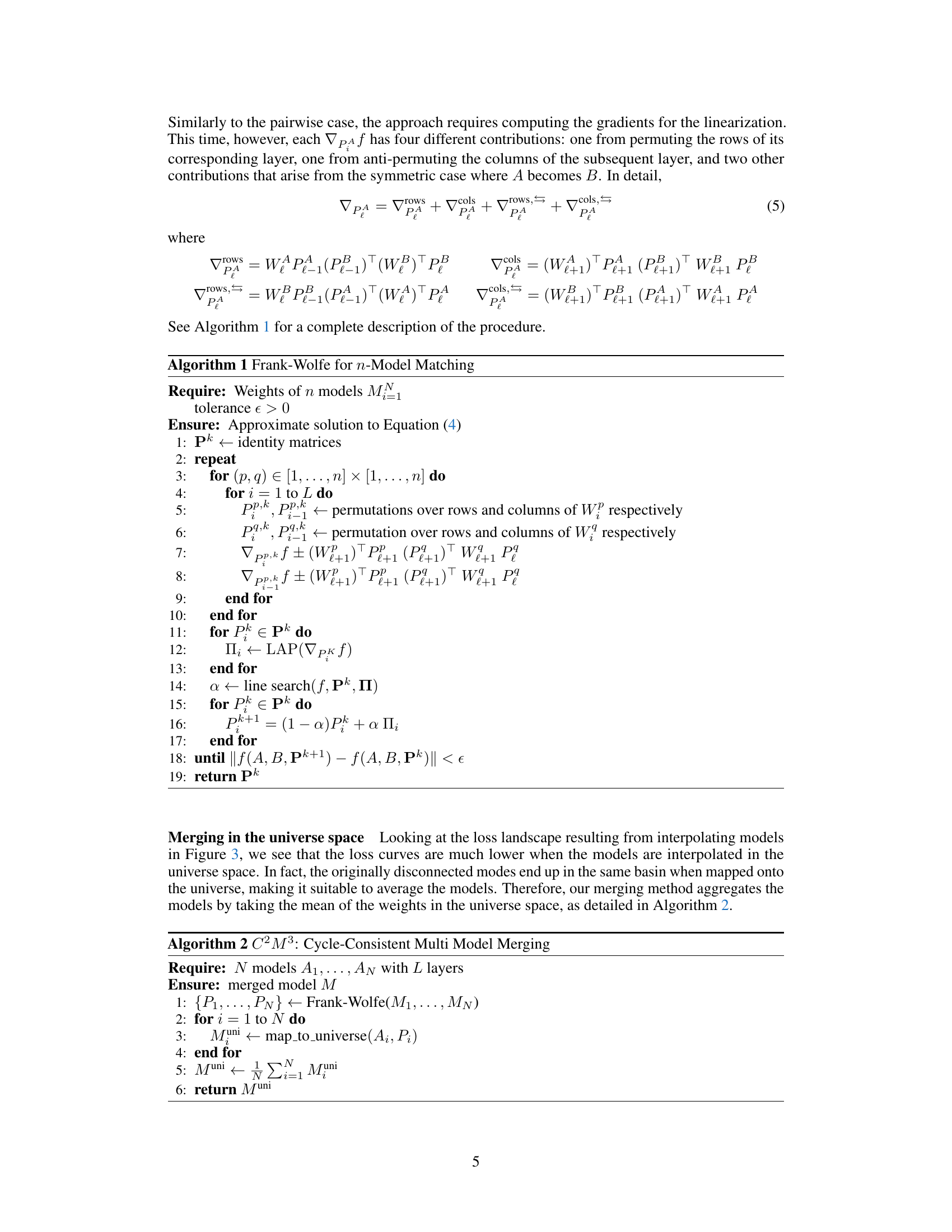
The Frank-Wolfe matching algorithm, as presented in the context of multi-model merging, offers a compelling approach to aligning neural networks by optimizing neuron permutations across all layers. Unlike pairwise methods, which often suffer from cycle inconsistency issues, this technique leverages the Frank-Wolfe algorithm to iteratively refine the global assignment of neurons, resulting in a more coherent and stable mapping between models. By factoring each permutation into mappings through a common “universe” space, cycle consistency is inherently enforced. The iterative nature, coupled with the computation of gradients reflecting inter-layer dependencies, contributes to the algorithm’s robustness and its ability to achieve a better global alignment. This is in contrast to layer-wise methods that struggle with accumulating error and variance across layers. The global optimization is key to addressing the limitations of the pairwise approach, enhancing the quality and reliability of multi-model merging.
Universe Space Merging#
The concept of “Universe Space Merging” in the context of the provided research paper appears to be a novel approach to neural network model aggregation. The core idea revolves around mapping the internal representations (neuron weights) of multiple models into a shared, common space – the “universe.” This mapping is done using carefully optimized permutations of the neurons within each model, ensuring consistency and preventing error accumulation during the merging process. The key innovation lies in enforcing cycle consistency, allowing for the composition of multiple model permutations within the universe space without introducing errors, thus facilitating seamless model merging. This method is distinct from pairwise approaches that lack this global constraint. Finally, the process of merging itself happens in this universe space, producing a final model that incorporates the salient features of the original models more effectively than methods relying solely on averaging or pairwise mappings.
Mode Connectivity#
Mode connectivity, a core concept in the paper, explores the geometric landscape of neural network loss functions. It challenges the traditional view of isolated minima (modes) by demonstrating the existence of low-energy paths connecting them. This connectivity is crucial because it implies that functionally equivalent networks may exist, differing only in the permutation of neurons. The paper highlights the importance of considering these symmetries during model merging, arguing that approaches neglecting these symmetries can lead to inconsistent results. The concept of mode connectivity is foundational to the paper’s proposed cycle-consistent multi-model merging method, which leverages the understanding of mode connectivity to ensure consistent results regardless of the order in which models are merged. This is achieved by mapping all models to a common ‘universe’ space, thus mitigating errors that accumulate from sequential pairwise merging. The research empirically investigates the influence of factors like network width and the number of models being merged on the overall performance and mode connectivity.
Merging Limitations#
The limitations of multi-model merging methods center around several key challenges. Cycle consistency, while theoretically desirable, can be difficult to achieve perfectly in practice, leading to accumulated errors when composing multiple pairwise mappings. Data-free methods, while avoiding the need for extra data, rely heavily on intrinsic model properties for alignment, making their performance sensitive to architectural choices and training dynamics. Linear mode connectivity, a crucial assumption underlying many merging strategies, is not always guaranteed, especially in wider networks, reducing the effectiveness of linear interpolation. Further, activation mismatch between models presents a hurdle, even after successful weight alignment. Generalization across diverse model architectures and datasets remains a significant limitation. Lastly, the computational cost associated with finding optimal permutations across multiple models grows considerably with increased model size and the number of models, a critical constraint for practical application.
More visual insights#
More on figures

This figure shows a 2D projection of the loss landscape for three models (A, B, C) before and after mapping them to a common ‘universe’ space using the proposed Cycle-Consistent Multi-Model Merging (C2M³) method. The left panel shows the original loss landscapes, demonstrating that the models reside in separate basins. The right panel depicts the same models after being mapped to the universe space. Notably, their loss landscapes now overlap significantly, indicating that the models reside within the same basin in the universe space. This illustrates the core concept of C2M³, which uses the universe space as a bridge to ensure cycle-consistency and facilitates effective model merging.

This figure shows a 2D projection of the loss landscape for three models (ΘA, ΘB, ΘC) before and after being mapped to a common space called the ‘universe’. The colors represent the loss values, with red indicating low loss and blue indicating high loss. Before mapping, the models are in different basins (separate low-loss regions). After mapping to the universe space using the proposed method, all three models (π(ΘA), π(ΘB), π(ΘC)) are located in the same basin, demonstrating the effectiveness of the method in aligning models.
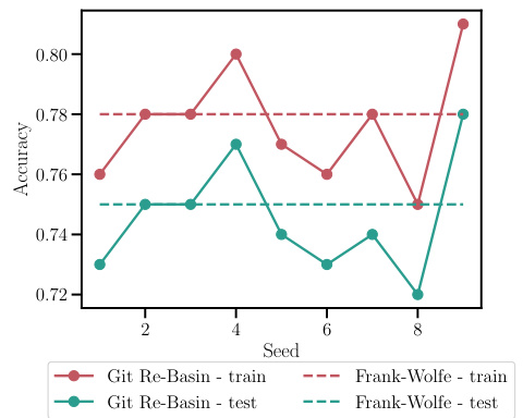
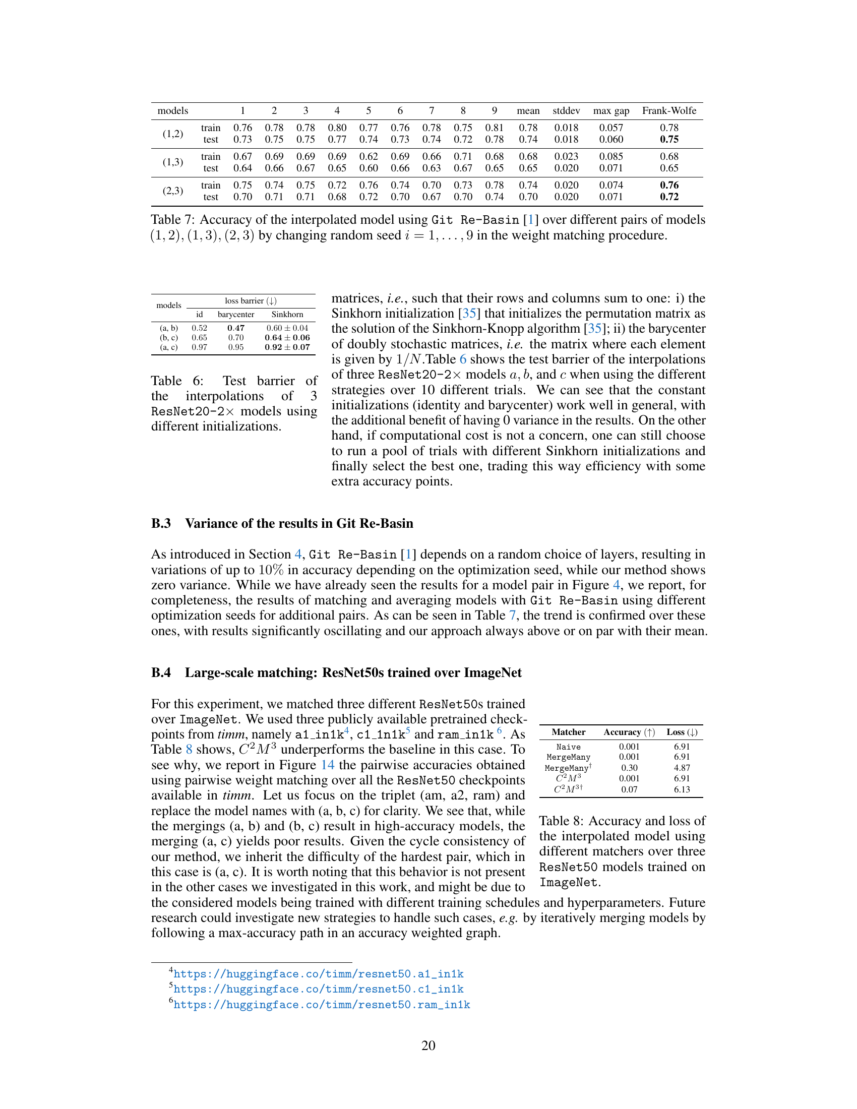
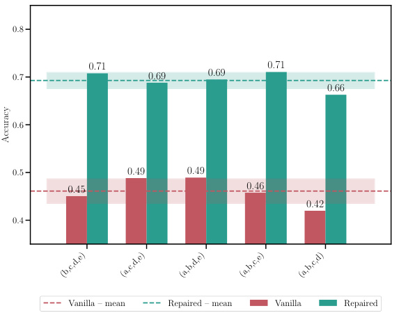
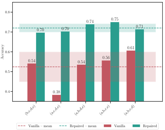
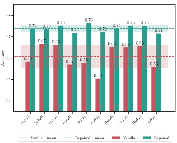
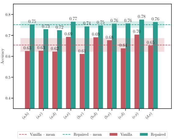
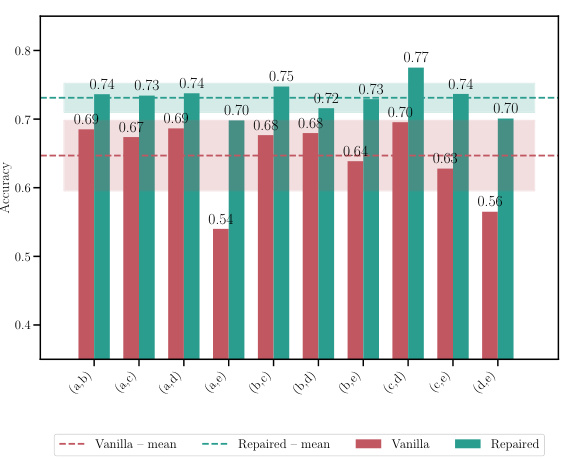
This figure shows the accuracy of a model obtained by interpolating two models using the Git Re-Basin method. The results are shown for different random optimization seeds. The goal is to demonstrate the impact of the random seed on the performance of the Git Re-Basin method.

This figure shows a 2D projection of the loss landscape for three models (ΘA, ΘB, ΘC) before and after mapping them to a common space called the ‘universe’. The colors represent the loss values, with red indicating low loss and blue indicating high loss. Before the mapping, the models are in separate basins (low-loss regions), indicating they are isolated. After mapping to the universe, the models are in the same basin, demonstrating that the mapping successfully aligns them.

This figure shows a 2D projection of the loss landscape for three models (ΘA, ΘB, ΘC) before and after they are mapped to a common space called the ‘universe’. The colors represent the loss value, with red indicating low loss (basins) and blue indicating high loss. Before mapping, the models are in separate basins, but after mapping to the universe space, they all lie within the same basin, indicating better mode connectivity.

This figure shows a 2D projection of the loss landscape for three models (A, B, C) before and after they are mapped to a common space called the ‘universe’. The left panel shows the original loss landscape where each model is in a separate basin. The right panel shows the loss landscape after the models have been mapped to the universe space, where all three models are located in the same basin. The redder zones indicate lower loss (better regions) and bluer zones indicate higher loss. This illustrates the concept of using a common space to align the models and merge them more effectively.

This figure visualizes the loss landscape before and after applying a transformation (mapping to the universe) to three models (ΘA, ΘB, ΘC). The left panel (a) shows the original landscape where the models are in separate basins (high-energy barriers). The right panel (b) shows the landscape after the transformation, where the transformed models (π(ΘA), π(ΘB), π(ΘC)) now reside within the same basin (low-energy region). This demonstrates that cycle-consistent multi-model merging successfully aligns the models into a common space.
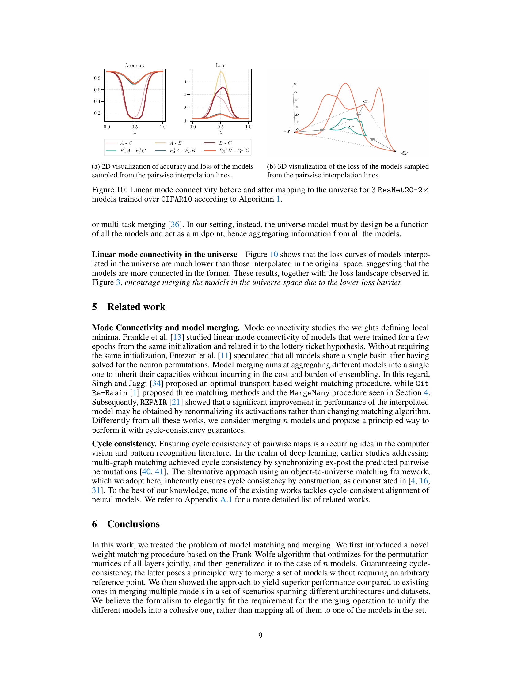
This figure shows a 2D projection of the loss landscape for three models (A, B, and C) before and after mapping them to a common ‘universe’ space. The left panel (a) shows the loss landscape for ResNet20 models trained on CIFAR100, while the right panel (b) shows the loss landscape for MLP models trained on MNIST. Before the mapping, the models are in separate basins (red regions indicate low-loss areas corresponding to local minima or basins), separated by high-energy barriers (blue regions indicate high-loss areas). However, after mapping to the universe space using the proposed Cycle-Consistent Multi-Model Merging (C2M³) method, the three models are now located in the same basin, indicating improved mode connectivity.

This figure visualizes the loss landscape before and after applying a transformation to map models into a shared ‘universe’ space. The left panel (a) shows the loss landscape for ResNet20 on CIFAR100, and the right panel (b) shows the loss landscape for an MLP on MNIST. In both cases, the models (ΘA, ΘB, ΘC) initially occupy distinct basins (low-loss regions shown in red). After the transformation (resulting in models π(ΘA), π(ΘΒ), π(Θc) in the universe space), the models are all located within a single basin, indicating a higher degree of connectivity. The visualization highlights how the proposed method improves the connectivity of different models by aligning them in the universe space.

This figure shows the loss landscape of three models before and after being mapped to a shared ‘universe’ space. Before mapping (left), the models occupy distinct basins (low-loss regions) implying isolation. After mapping to the universe space (right), all models reside within the same basin indicating that they are now connected. This visualizes the core concept of cycle-consistent multi-model merging where models are first mapped to a common space before being averaged.
This figure shows a 2D projection of the loss landscape for three models (A, B, and C) before and after being mapped to a common ‘universe’ space. The colors represent the loss values, with red indicating low loss (basins) and blue indicating high loss. Before the mapping, the models are in separate basins, implying isolated minima. However, after mapping to the universe space using the proposed cycle-consistent method, the models are all located within the same basin, illustrating the success of the approach in aligning the models.
This figure shows a 2D projection of the loss landscape for three models (A, B, and C) before and after applying a transformation that maps them to a common ‘universe’ space. The visualization helps illustrate the concept of cycle consistency in multi-model merging. Before the transformation, the models are in separate basins (low-loss regions). After mapping to the universe space, the transformed models (π(ΘA), π(ΘB), π(ΘC)) reside within the same basin, indicating that the method effectively aligns the models by finding consistent permutations across layers.

This figure shows a 2D projection of the loss landscape for three models (A, B, C) before and after being mapped to a common ‘universe’ space. The colormap represents the loss values, with red indicating low loss (basins) and blue indicating high loss. Before mapping, the models are in different basins, suggesting isolation. After mapping to the universe space via a learned transformation, all three models reside in the same basin, indicating that the models’ respective modes (low-loss regions) have been brought into proximity. This demonstrates the effectiveness of the proposed Cycle-Consistent Multi-Model Merging (C2M³) method in aligning models.
This figure shows a 2D projection of the loss landscape for three models (ΘA, ΘB, ΘC) before and after mapping them to a common ‘universe’ space using the proposed Cycle-Consistent Multi-Model Merging (C2M³) method. The left panel shows the original models, which are in separate basins (low-loss regions). The right panel shows the models after mapping to the universe, demonstrating that the models now reside within the same basin, indicating successful alignment and mode connectivity.

This figure visualizes the loss landscape before and after applying a transformation to map models into a common ‘universe’ space. The left panel (a) shows the original loss landscape for three models (ΘA, ΘB, ΘC), illustrating separate basins. The right panel (b) shows the loss landscape after the transformation (π(ΘA), π(ΘB), π(ΘC)), demonstrating that the models now reside within the same basin in the universe space. The color scheme uses red for low-loss areas and blue for high-loss areas.
This figure visualizes the loss landscapes before and after applying a transformation to a common ‘universe’ space. It shows that, in the original space, the three models (ΘA, ΘB, ΘC) are in separate basins (low-loss regions). After mapping them to the universe space using a transformation (represented by π), all three models (π(ΘΑ), π(ΘΒ), π(Θc)) now reside in the same basin, indicating a more connected and unified representation.
This figure shows a 2D projection of the loss landscape for three models (ΘA, ΘB, ΘC) before and after being mapped to a common ‘universe’ space. The mapping process aims to align the models by finding optimal permutations of their neurons. Before mapping, the models are located in separate basins (low-loss regions), indicating isolation. After mapping to the universe, the models’ corresponding images (π(ΘA), π(ΘB), π(ΘC)) are all found in the same basin. The plot visually demonstrates how the proposed method successfully connects and merges the models into a common region, highlighting improved mode connectivity.
This figure shows a 2D projection of the loss landscape for three models (ΘA, ΘB, ΘC) before and after mapping them to a common ‘universe’ space (π(ΘA), π(ΘB), π(ΘC)). The colormap represents the loss value, with red indicating low loss and blue indicating high loss. Before the mapping, the models are in separate basins (low-loss regions). After mapping to the universe space, all three models are clustered together in a single basin, indicating that the universe space successfully aligns the models.
This figure shows a 2D projection of the loss landscape for three models (ΘA, ΘB, ΘC) before and after being mapped to a common ‘universe’ space. Before mapping, the models are in separate basins (low-loss regions), indicating isolation. After mapping to the universe, all three models (π(ΘA), π(ΘB), π(ΘC)) are located in the same basin, demonstrating that the proposed cycle-consistent method effectively aligns the models.

This figure visualizes the loss landscape before and after mapping models to a common ‘universe’ space. It shows that in the original space (left), the three models (A, B, C) reside in distinct basins, separated by high-energy barriers. However, after transforming the models to the universe space (right), they are all situated in the same basin, indicating improved connectivity and facilitating the merging process.
This figure shows a 2D projection of the loss landscape for three models (ΘA, ΘB, ΘC) before and after being mapped to a shared ‘universe’ space using the proposed Cycle-Consistent Multi-Model Merging method. The left panel shows the original models, demonstrating that they reside in separate basins (low-loss regions). The right panel shows the models after being mapped to the universe space, highlighting that they now all reside within the same basin. This visually demonstrates the method’s ability to align models from different loss landscapes, facilitating subsequent merging.
This figure shows a 2D projection of the loss landscape for three models (ΘA, ΘB, ΘC) before and after mapping them to a common ‘universe’ space (π(ΘA), π(ΘB), π(ΘC)). The color scheme represents the loss value, with red indicating low loss (likely basins) and blue representing high loss. The key observation is that after mapping to the universe space, the three models now reside in the same basin, suggesting a successful alignment by the proposed method.
This figure shows a 2D projection of the loss landscape for three models (ΘA, ΘB, ΘC) before and after they are mapped to a common ‘universe’ space using the proposed cycle-consistent multi-model merging method. The red regions represent low-loss areas (basins), and blue regions represent high-loss areas. The key observation is that after mapping to the universe space (right), all three models are located within the same low-loss basin, highlighting the effectiveness of the proposed method in aligning the models and eliminating the mode isolation problem.
More on tables
This table shows the accuracy and loss of merged models resulting from merging 5 models with different initializations. It compares the performance of the proposed C2M³ method with a naive averaging approach and the MergeMany algorithm. The results are presented for different architectures (MLP, ResNet, VGG16) and datasets (EMNIST, CIFAR10, CIFAR100). The best results for each configuration are highlighted in bold. The ‘+’ symbol indicates that REPAIR (activation renormalization) was applied to the merged model. The table highlights the consistent improvement in accuracy and reduction in loss achieved by C2M³ compared to the baseline methods.

This table presents the accuracy and loss of the merged model obtained by merging five models trained with different initializations using different model merging methods: Naive averaging, MergeMany, C2M³, and C2M³ with the REPAIR post-processing technique. The results are shown for various datasets and model architectures (MLP, ResNet, and VGG16). The table highlights the superiority of the C2M³ approach, especially when combined with REPAIR, in achieving higher accuracy and lower loss compared to other methods. It demonstrates the effectiveness of the proposed cycle-consistent multi-model merging method in improving model performance.

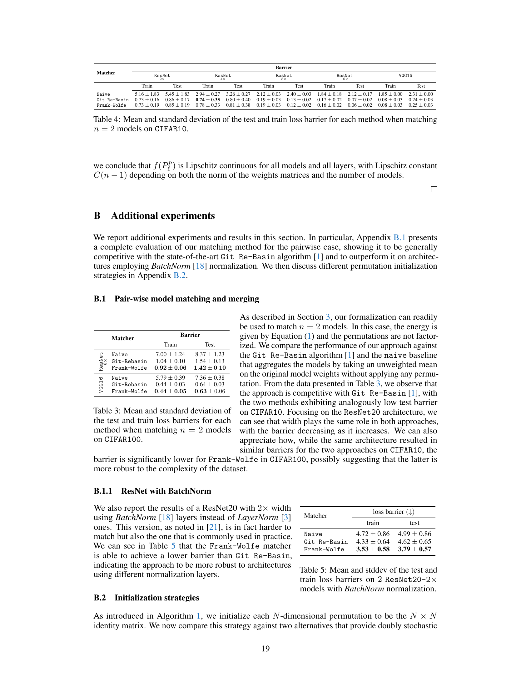
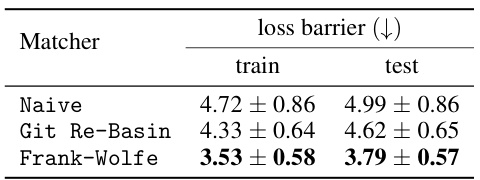
This table shows the mean and standard deviation of the training and testing loss barriers for different model matching methods on the CIFAR100 dataset. Three methods are compared: a naive averaging method, the Git Re-Basin method, and the Frank-Wolfe method proposed in the paper. The results indicate the performance of each method in aligning two models by measuring the loss barrier between them.
This table shows the accuracy and loss of merged models trained with different initializations, comparing the proposed C2M³ method against baselines. It highlights the improvement achieved by C2M³ and the effect of post-processing using the REPAIR method.

This table shows the accuracy and loss for a merged model created using different methods. Five models were initially trained with different initializations. The methods compared include a naive averaging of weights, the MergeMany approach, and the proposed C2M³ approach, both with and without activation renormalization (REPAIR). The results are shown for various architectures (MLP, ResNet, VGG16) and datasets (EMNIST, CIFAR10, CIFAR100). The best results for each scenario are bolded, highlighting the effectiveness of the C2M³ method, particularly when coupled with REPAIR.

This table presents the test barrier values obtained when interpolating between three ResNet20 models with 2x width using different initialization strategies for the permutation matrices: identity matrix (id), barycenter of doubly stochastic matrices (barycenter), and Sinkhorn initialization (Sinkhorn). The results show that the constant initializations (identity and barycenter) perform reasonably well, offering the added benefit of zero variance in results. However, if computation cost is not an issue, running multiple trials with Sinkhorn initialization and selecting the best result could potentially improve accuracy slightly, though this trades efficiency for marginal gains.
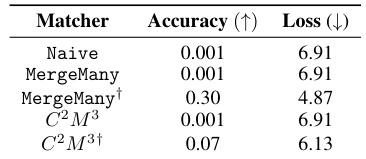
This table presents the accuracy and loss values achieved by different model merging methods on various datasets when merging 5 models with different initializations. The methods compared include a naive averaging of weights, the MergeMany approach, and the proposed C2M³ approach, both with and without activation renormalization (REPAIR). The table highlights the superior performance of the C2M³ method, especially when coupled with REPAIR, showcasing its ability to effectively merge models trained with diverse initializations while achieving better accuracy and lower loss than existing methods.

This table compares the accuracy and loss of a merged model created using different methods, including a naive averaging approach, the MergeMany approach, and the proposed C2M³ method, both with and without activation renormalization (REPAIR). Five models, each trained with different initializations, are merged. The results show that C2M³ significantly outperforms the other methods in terms of accuracy and loss, particularly when REPAIR is applied.

This table presents the accuracy and loss of models obtained by merging five models that were trained with different initializations. The results are compared for different architectures (MLP, ResNet, and VGG16) on different datasets (EMNIST, CIFAR10, and CIFAR100). Two different merging methods are shown: C2M³ and MergeMany. A naive approach (averaging weights without any matching) is also included as a baseline. The table shows that C2M³ consistently outperforms both the MergeMany algorithm and the naive baseline in terms of accuracy and loss. It also shows that applying the REPAIR technique to the merged models can improve the results further.
Full paper#
