↗ OpenReview ↗ NeurIPS Homepage ↗ Chat
TL;DR#
Many real-world applications require neural networks to continuously learn from new data, often using warm-starting (initializing training with previously learned weights). However, this frequently leads to
plasticity loss: the network’s reduced ability to learn new information. This paper investigates this problem, even under stationary data distributions (where data characteristics remain constant). The core issue identified is the memorization of noise during the process of warm-starting, which hinders the network’s ability to adapt to new data.
To address this, the researchers introduce DASH (Direction-Aware SHrinking), a new method designed to mitigate plasticity loss. DASH works by selectively forgetting the noise while preserving the already learned useful features, effectively resolving the conflict between using past knowledge and having the capability to learn new things. Through experiments, they verify that DASH effectively improves test accuracy and training efficiency on various tasks, demonstrating the method’s efficacy and potential to significantly impact continual learning and real-world applications.
Key Takeaways#
Why does it matter?#
This paper is crucial for researchers in deep learning and continual learning. It addresses the critical issue of plasticity loss during warm-starting, a common practice in real-world applications. The proposed DASH method offers a practical solution and the theoretical framework provides insights into the underlying mechanisms of plasticity loss, opening new avenues for research in overcoming this limitation and improving model adaptability.
Visual Insights#

This figure compares the performance of different training methods (Cold, Warm, S&P, and DASH) on the Tiny-ImageNet dataset using ResNet-18. The x-axis represents the number of experiments, where each experiment adds a chunk of data to the training set. The left plot shows test accuracy, illustrating that DASH consistently outperforms other methods, especially warm-starting which often performs worse than training from scratch. The right plot shows the number of training steps for each experiment, highlighting DASH’s efficiency in reaching convergence.
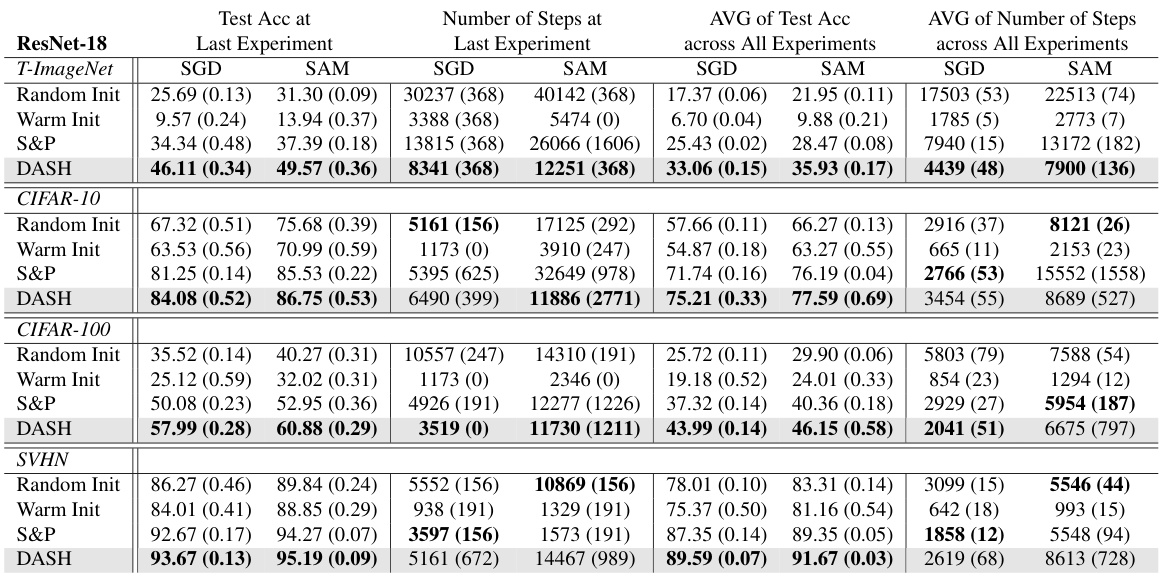
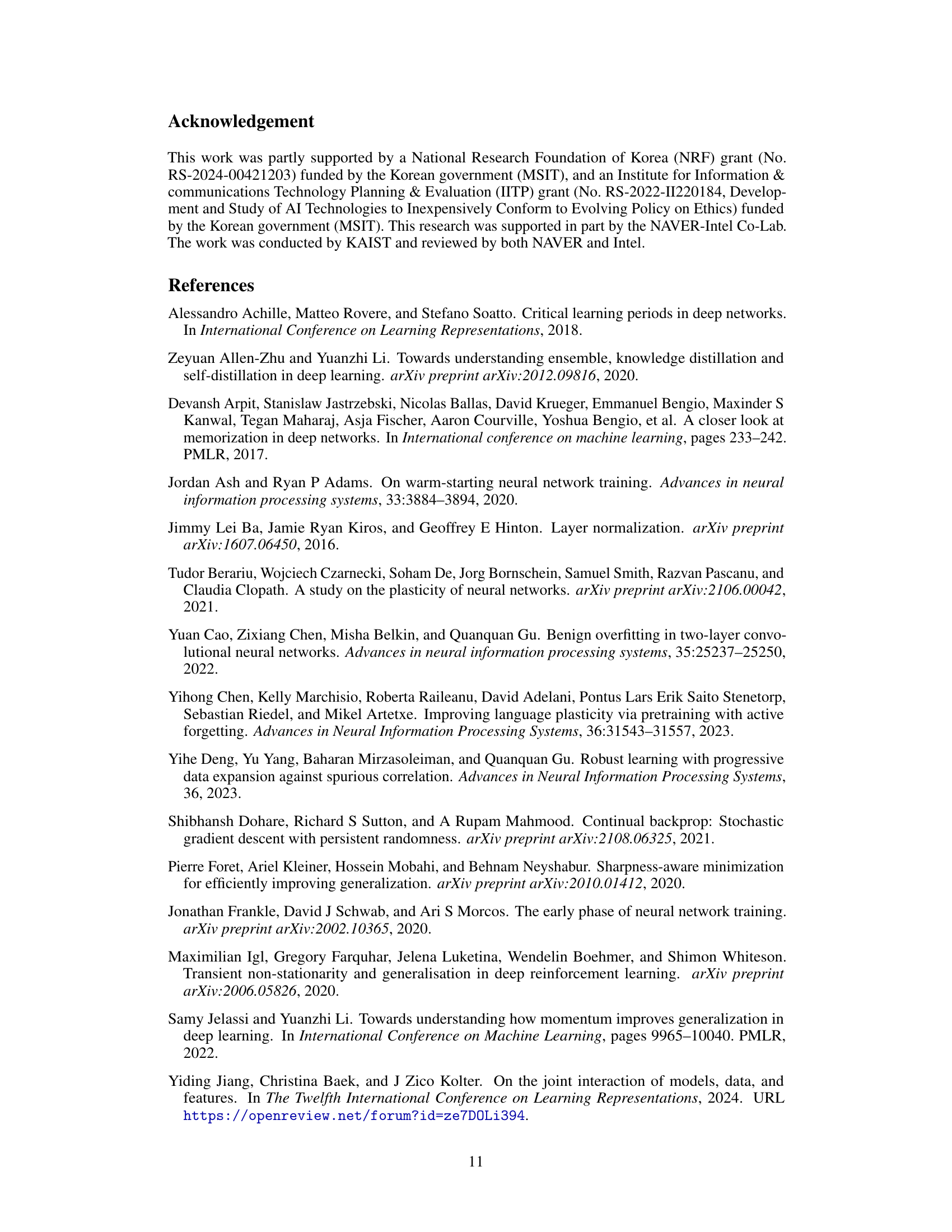
This table presents a comparison of different neural network training methods (random initialization, warm-starting, Shrink & Perturb, and DASH) across four datasets (Tiny-ImageNet, CIFAR-10, CIFAR-100, and SVHN) using ResNet-18. For each dataset and method, it reports the test accuracy achieved at the last experiment and the average test accuracy across all experiments, along with the number of steps taken in the last experiment and the average number of steps across all experiments. Bold values highlight the best-performing method for each metric. The table demonstrates the impact of different warm-starting strategies on model performance and training efficiency.
In-depth insights#
Plasticity Loss Issue#
The phenomenon of plasticity loss in neural networks, particularly during warm-starting, presents a significant challenge. Warm-starting, initializing a network with pre-trained weights, is appealing for continuous learning scenarios, but often results in a reduced ability to learn new information. This is not solely restricted to non-stationary data distributions, as the paper highlights a surprising loss of plasticity even under stationary conditions. This counter-intuitive observation necessitates a deeper investigation into the underlying mechanisms. The core issue appears to be noise memorization, where the network prioritizes memorizing noisy data rather than extracting meaningful features. The proposed DASH method directly addresses this limitation by strategically shrinking weight vectors, selectively forgetting memorized noise while preserving learned features. This approach effectively combats the overfitting that often hinders generalization performance during warm-starting, leading to improved accuracy and training efficiency. The paper’s framework for understanding and mitigating this issue is valuable for practical applications of continuous neural network learning.
DASH Framework#
The DASH framework, introduced to address the issue of plasticity loss in warm-started neural network training, offers a novel approach to selectively forget noise while preserving learned features. It combines elements of feature learning frameworks, acknowledging the presence of both label-relevant features and label-irrelevant noise in data. DASH’s core innovation lies in its direction-aware shrinking technique. Instead of uniformly shrinking weights, it selectively reduces the magnitude of weights based on their alignment with the negative gradient of the loss function. Weights aligned with the gradient (representing learned features) are shrunk less aggressively, while weights misaligned (memorized noise) are shrunk more strongly. This selective forgetting mechanism allows the model to adapt to new information without catastrophic forgetting, improving its generalization performance. The framework’s discrete learning process, which emphasizes sequential learning of high-frequency features before noise memorization, provides valuable insights into the underlying dynamics of warm-starting. While the experimental results are promising, future work could focus on extending the framework’s theoretical analysis to more complex scenarios. DASH also highlights the importance of striking a balance between retaining useful knowledge and forgetting noise for efficient and effective neural network training.
Stationary Case Study#
A stationary case study in the context of neural network warm-starting would involve training a model on a dataset drawn from a fixed, unchanging data distribution. The core question is whether warm-starting (initializing with pre-trained weights) hinders the model’s ability to learn new information compared to training from scratch (cold-starting). A key aspect would be to isolate the effects of noise memorization in the pre-trained weights. The study would ideally compare the generalization performance of warm-started and cold-started models on unseen data, looking for evidence of reduced plasticity (the ability to adapt to new information) in the warm-started case. The ideal scenario would show that the cold-started model outperforms the warm-started model because the initial weights may hinder learning. This could be due to the model becoming stuck in suboptimal regions of the loss landscape or to overfitting to noise present in the initial training data. Such a study helps quantify the negative effect of warm-starting in situations where the data distribution remains constant, which is important for understanding and mitigating the ’loss of plasticity’ phenomenon.
Direction-Aware Shrink#
The concept of “Direction-Aware Shrink” suggests a method for refining model weights during neural network training, particularly beneficial in warm-starting scenarios. Instead of uniformly shrinking all weights, which risks losing valuable learned features, this approach selectively shrinks weights based on their alignment with the negative gradient of the loss function. Weights strongly aligned with the negative gradient (indicating a significant contribution to the error) are shrunk more aggressively, effectively forgetting noise and potentially harmful memorized information. Conversely, weights aligned with the gradient (representing valuable, previously learned features) are shrunk less, preserving crucial aspects of the model’s knowledge. This directionality provides a more nuanced approach to regularization, preventing catastrophic forgetting and improving the model’s adaptability to new data without sacrificing learned information. This approach is particularly valuable in contexts such as continual learning, where the model is continuously exposed to new data and maintaining plasticity is crucial. The technique aims to balance the benefits of warm-starting (faster convergence) with those of cold-starting (better generalization) by selectively preserving relevant information while forgetting noise.
Future Research#
Future research directions stemming from this paper could explore extending the theoretical framework to encompass more complex scenarios, such as non-stationary data distributions often encountered in reinforcement learning or continual learning. A deeper investigation into the interplay between noise memorization and the Hessian rank of the training objective would provide a more comprehensive understanding of plasticity loss. The efficacy of DASH in diverse architectures and datasets beyond those tested warrants further exploration. Analyzing the impact of different noise types and strengths on feature learning would refine the understanding of noise memorization’s role. Finally, developing a more robust and efficient method for selectively forgetting noise while preserving learned features remains a key area for future research. This might involve exploring alternative shrinkage strategies or incorporating more sophisticated methods for identifying and mitigating noise.
More visual insights#
More on figures

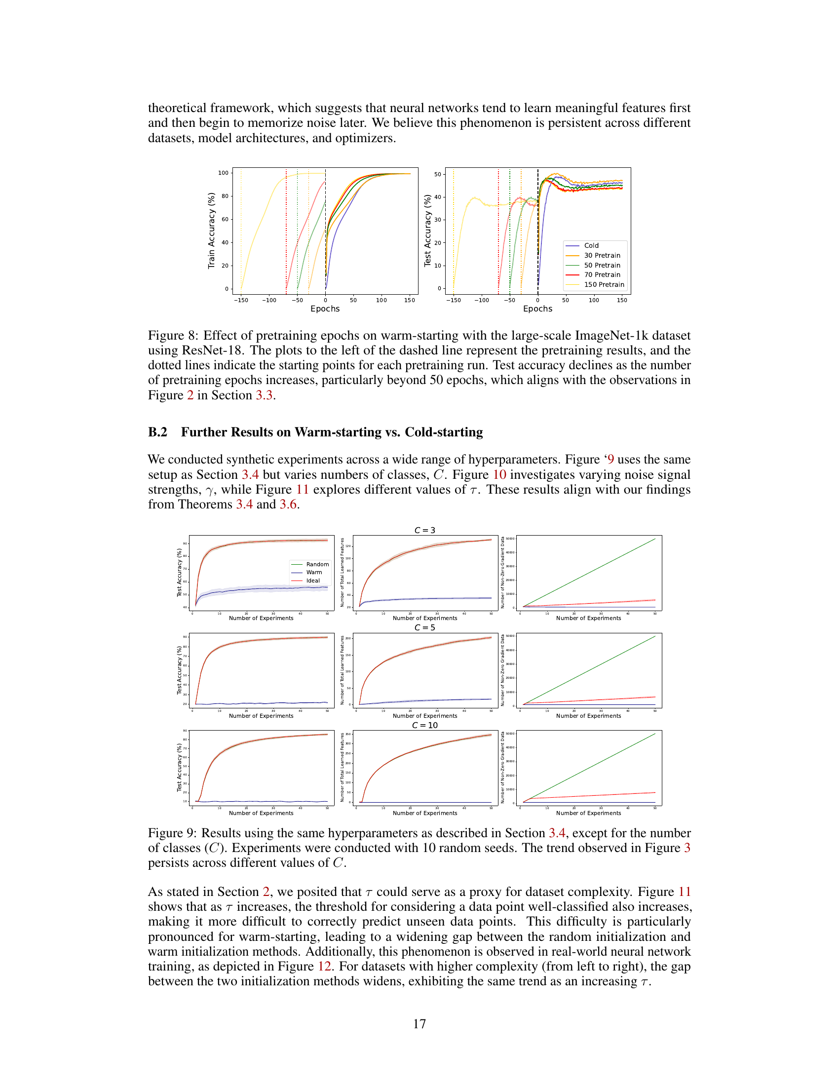
This figure shows the test accuracy results of three-layer MLP and ResNet-18 models when pretrained for varying epochs and then fine-tuned on the full dataset. It compares the performance of warm-starting (pre-training then training) with cold-starting (training from scratch). The plot includes train accuracy during the pre-training phase. The results show that if the pre-training is stopped at a certain point and fine-tuned on full data, the test accuracy is maintained. However, if the pre-training continues beyond the specific threshold, then warm-starting significantly impairs the model’s performance, which indicates noise memorization during excessive pre-training.

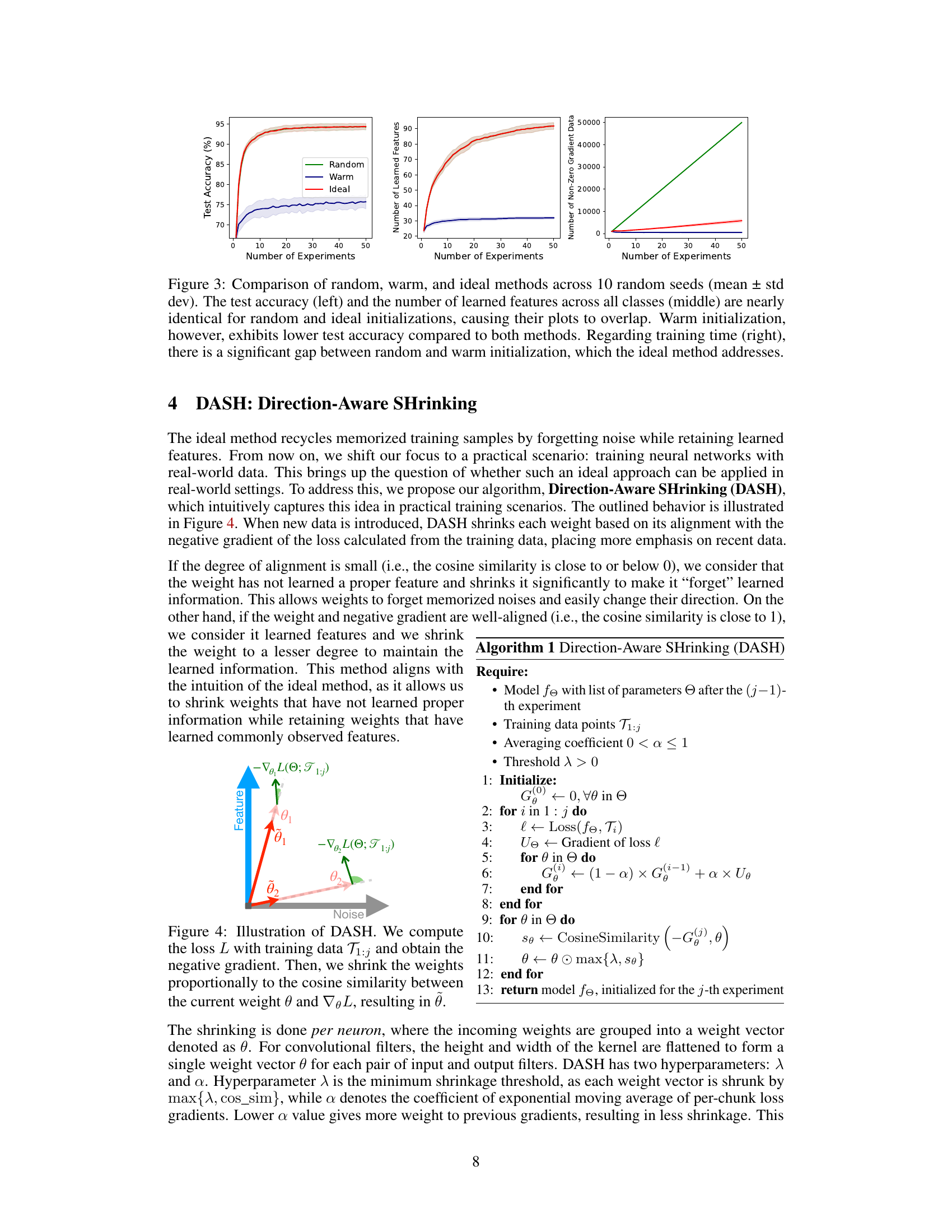
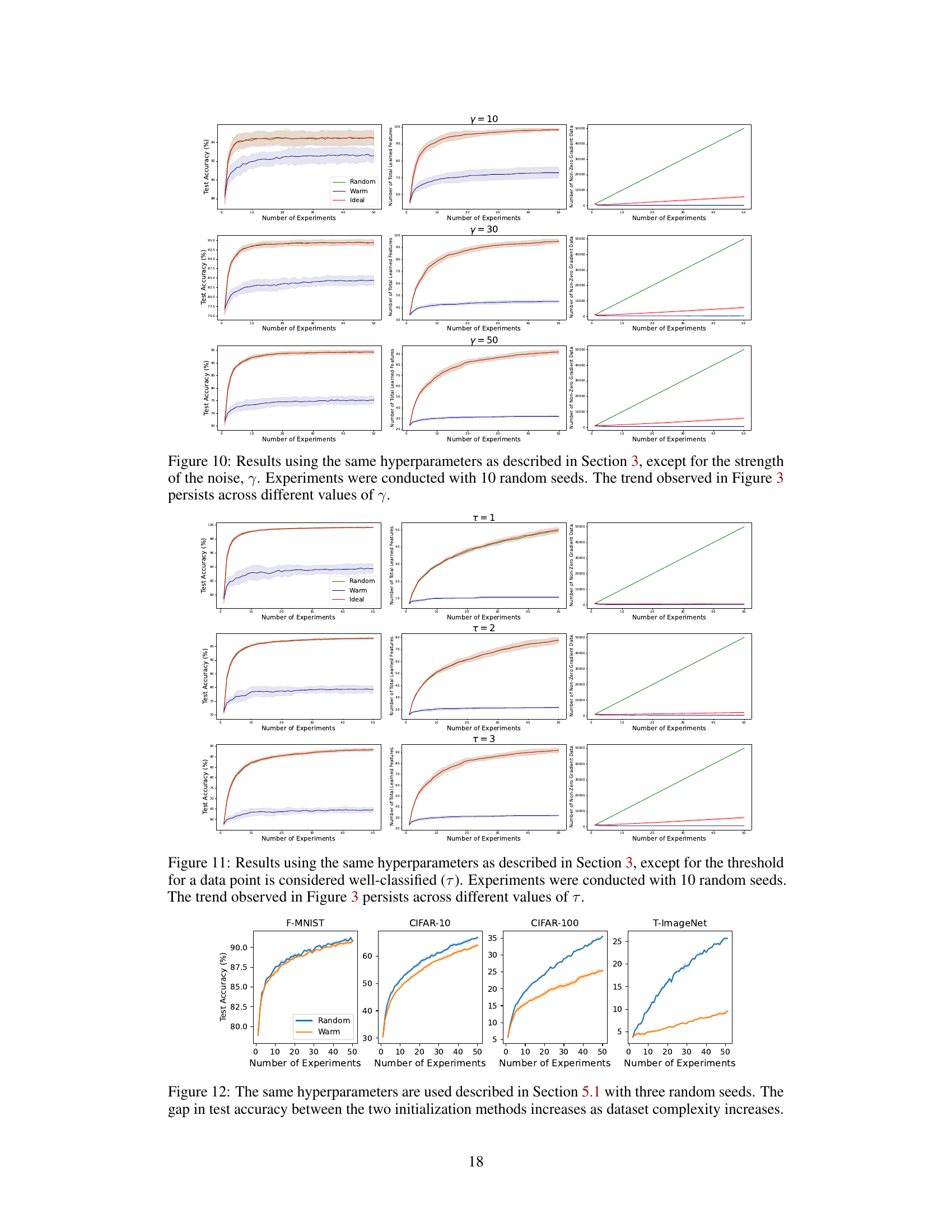
This figure compares the performance of three different initialization methods (random, warm, and ideal) across 50 experiments on a dataset. The plots show test accuracy, the number of learned features, and the number of non-zero gradient data points. The results indicate that warm-starting results in significantly worse test accuracy than both random initialization (cold-starting) and the ideal method, while the ideal method demonstrates that retaining learned features and forgetting noise leads to better performance compared to cold-starting, albeit with increased training time. The warm-starting method results in a smaller number of learned features, suggesting that memorization of noise impairs performance.

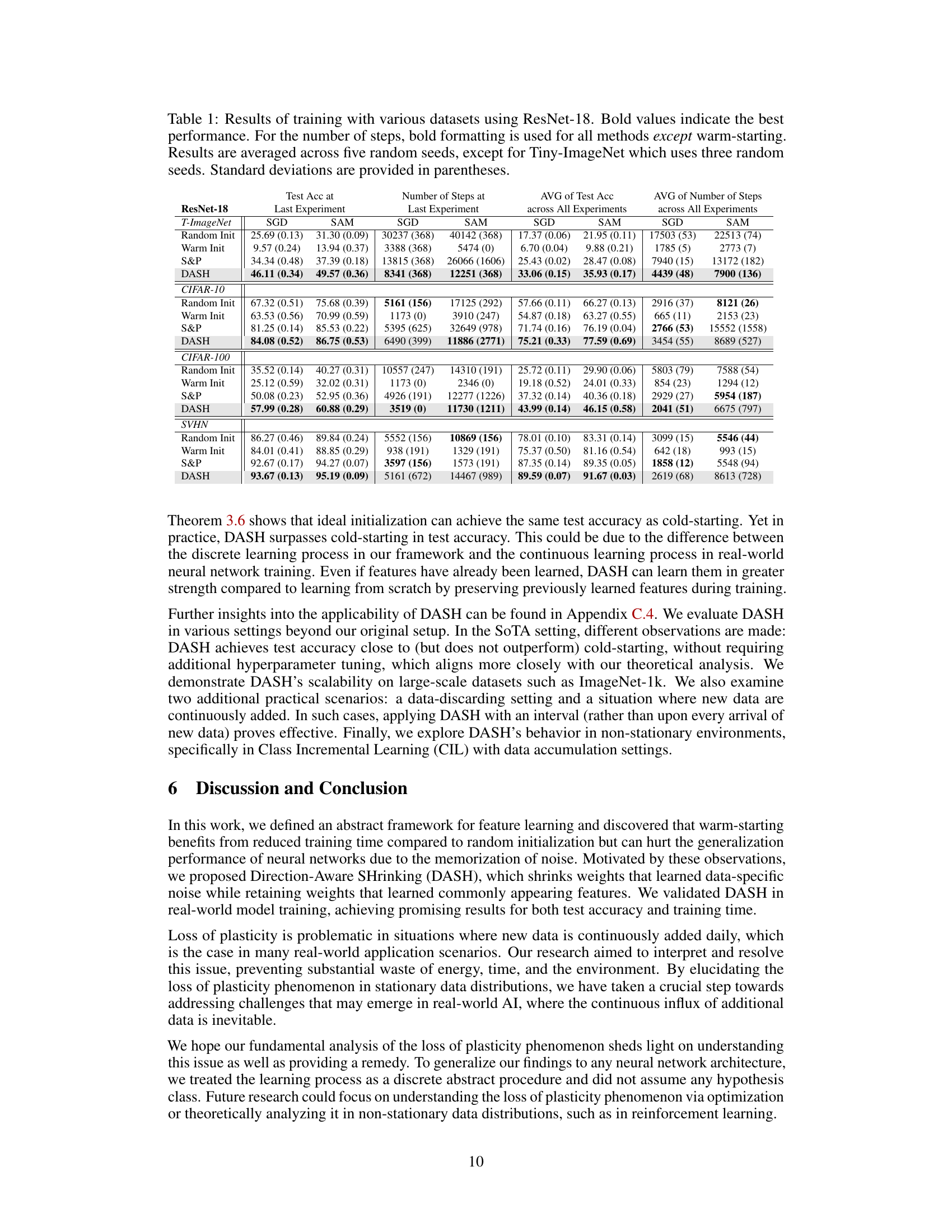
This figure illustrates the core concept of the DASH algorithm. It shows how weights are shrunk based on their alignment with the negative gradient of the loss function. Weights that align well with the negative gradient (representing learned features) are shrunk less, while those that don’t align well (representing noise) are shrunk more. This selective forgetting of noise helps to prevent the loss of plasticity.

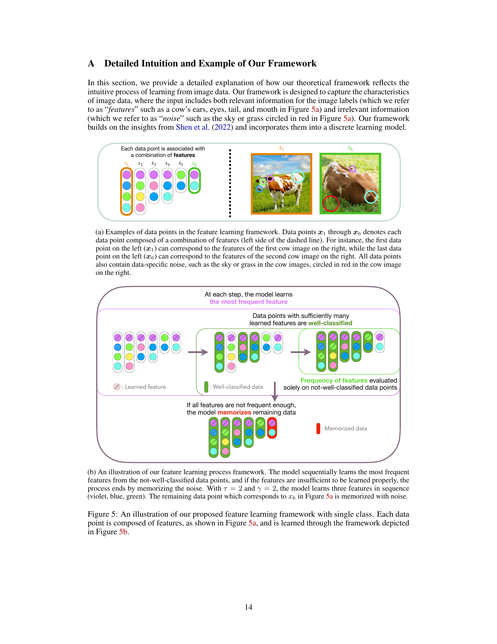
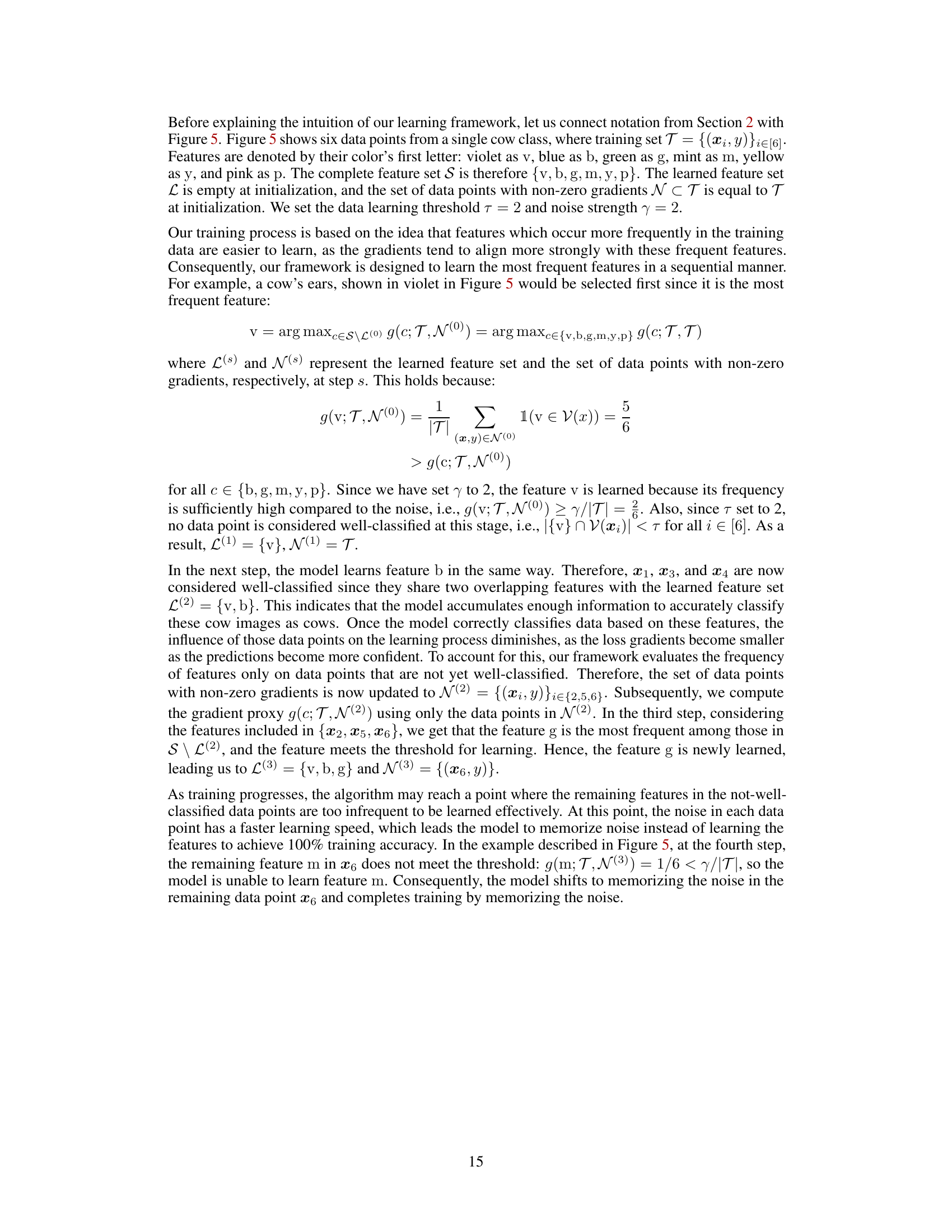
This figure illustrates the feature learning process using a simple example with a single class of images. Figure 5a shows data points (represented as vertical columns of colored dots) that are each a combination of class-relevant features (the colored dots) and class-irrelevant noise. Figure 5b depicts the learning process. The model sequentially selects and learns features from the data points based on their frequency, starting with the most frequent feature, until no features meet the learning threshold. Then the model begins memorizing the noise from the remaining data points. This illustrates the core idea of the proposed feature learning framework.

This figure compares the test accuracy and training efficiency of different neural network training methods on the Tiny-ImageNet dataset using ResNet-18. The methods include cold-starting (training from scratch), warm-starting (starting with pre-trained weights), Shrink & Perturb (S&P), and the proposed DASH method. The x-axis represents the number of experiments, each adding more data. The results show that DASH outperforms both cold-starting and warm-starting in terms of test accuracy while requiring fewer training steps.

This figure shows the relationship between the initial gradient norm of training data and the number of steps required for convergence in both warm-starting and cold-starting scenarios using ResNet-18 on CIFAR-10. The x-axis represents the initial gradient norm, which is a proxy for the complexity of the data (higher norm suggests more complex data). The y-axis represents the number of training steps needed for convergence. Each point represents a single experiment, with the color intensity indicating the number of experiments with similar values. It visually demonstrates how the number of training steps increases with increasing initial gradient norm, and also shows a difference between warm and random initializations.

This figure compares the performance of different neural network training methods on the Tiny-ImageNet dataset using ResNet-18. The experiment involves incrementally adding data in 50 chunks, training until 99.9% training accuracy is reached before adding the next chunk. The left graph shows test accuracy, while the right graph shows the number of training steps. The methods compared are cold-starting, warm-starting, Shrink & Perturb (S&P), and the proposed DASH method. DASH shows superior generalization performance and faster convergence compared to the other methods.

This figure compares the test accuracy of models trained with different pretraining durations on the full dataset. It shows that pre-training for an excessive number of epochs before fine-tuning on the full dataset hurts performance. The results suggest that an optimal pre-training duration exists, where exceeding that optimal duration leads to memorization of noise and poorer generalization ability. The experiment is conducted using both a three-layer MLP and a ResNet-18 model, each with multiple random seeds to assess variance.

This figure compares the performance of three different initialization methods: random (cold-start), warm-start, and an ideal method, across 10 random seeds. The left panel shows test accuracy, where both random and ideal initialization perform similarly and significantly better than warm-start. The middle panel shows the number of learned features across all classes, which are also similar for random and ideal but far fewer for warm start. The right panel shows training time (measured as the number of non-zero gradient data points). The ideal method significantly improves upon the warm-start training time, showing its efficiency. The results are averaged and the standard deviations are shown.

This figure compares the performance of three different initialization methods: random (cold-starting), warm-starting, and an ideal method (where only noise is forgotten). The results show that warm-starting performs significantly worse than random initialization and the ideal method in terms of test accuracy. However, warm-starting has a significantly shorter training time. The ideal method achieves the best accuracy and training time, indicating that retaining features while forgetting noise is crucial for efficient and accurate learning.

This figure compares the performance of three different initialization methods (random, warm, and ideal) across 50 experiments on a dataset that grows with each experiment. The left panel shows that cold-start (random) and ideal initialization achieve similar high test accuracy, while warm-starting performs significantly worse. The middle panel shows that the number of features learned is similar for both random and ideal initializations, and much lower for warm-starting, suggesting that warm-starting fails to learn new features effectively. The right panel shows that the training time (number of steps) is far less for warm-starting compared to cold-starting, with ideal initialization showing a training time between the two.

This figure compares the test accuracy and training efficiency (number of steps) of different methods on the Tiny-ImageNet dataset using ResNet-18. The dataset was incrementally added in chunks, and models were trained until 99.9% training accuracy before moving to the next chunk. The methods compared are cold-starting, warm-starting, Shrink & Perturb (S&P), and the proposed DASH method. DASH demonstrates superior generalization performance and training efficiency compared to the other approaches.

This figure compares the performance of different warm-starting methods against cold-starting on the Tiny-ImageNet dataset using ResNet-18. The x-axis represents the number of experiments (with data added incrementally), and the y-axis shows test accuracy and the number of training steps. DASH consistently outperforms warm-starting and S&P (Shrink & Perturb), demonstrating its effectiveness in maintaining plasticity. The right plot shows that DASH achieves comparable generalization performance while requiring fewer steps.
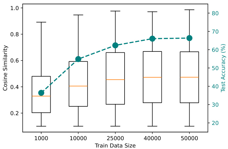
This figure shows the relationship between the cosine similarity of weights and negative gradients from the test data, and the test accuracy of a 3-layer CNN trained on CIFAR-10 with varying training data sizes. It supports the intuition behind DASH by visually demonstrating that higher cosine similarity (indicating weights have learned features) correlates with better test accuracy. The box plots show the distribution of cosine similarity values for each training data size, while the line graph illustrates the corresponding test accuracy.
This figure compares the performance of different neural network training methods on the Tiny-ImageNet dataset using ResNet-18. The x-axis represents the number of experiments, where in each experiment a new chunk of data is added to the training set. The y-axis on the left shows test accuracy and the y-axis on the right shows the number of training steps. The methods compared are cold-starting (training from scratch), warm-starting (initializing with pre-trained weights), Shrink & Perturb (S&P), and the proposed DASH method. The results demonstrate that DASH significantly outperforms other methods in generalization performance while requiring fewer training steps.

This figure compares the test accuracy and the number of training steps of different methods (Cold, Warm, S&P, DASH) on the Tiny-ImageNet dataset using ResNet-18. The dataset is incrementally expanded across 50 experiments. DASH shows improved test accuracy and training efficiency compared to other methods, especially warm-starting.

This figure compares the performance of three different initialization methods: random, warm, and ideal, across 10 random seeds. The results are presented for three metrics: test accuracy, the number of learned features, and training time. The random and ideal methods show nearly identical results for test accuracy and the number of learned features, while the warm method exhibits significantly lower test accuracy and a much shorter training time. The ideal initialization method bridges the gap between warm and random methods by achieving similar accuracy as the random method with similar training time to the warm method.
This figure compares the performance of three different initialization methods: random (cold-starting), warm-starting, and an ideal method. The results are averaged over 10 random seeds, and error bars show standard deviations. The left panel shows test accuracy, the middle panel shows the number of learned features, and the right panel shows training time (measured as number of steps or number of non-zero gradient data points). The key observation is that while warm starting leads to faster convergence (shorter training time), it results in significantly lower test accuracy than both cold starting and the ideal method. The ideal method achieves comparable test accuracy to cold-starting with a significantly reduced training time. This highlights the trade-off between speed and accuracy in warm-starting and shows the potential of the ideal method to improve generalization without sacrificing efficiency.
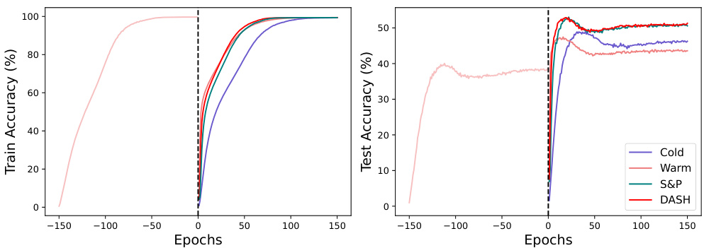
This figure compares the test accuracy of models trained using different initialization methods (random, warm-start, and the proposed DASH method) on the Tiny-ImageNet dataset. The x-axis shows the number of pre-training epochs, and the left y-axis shows the test accuracy after fine-tuning on the full dataset. The right y-axis shows the pre-training accuracy. The results show that warm-starting leads to worse performance than cold-starting if the pre-training is extended beyond a certain point, while DASH maintains high test accuracy.

The figure compares the test accuracy and training steps of different methods (Cold, Warm, S&P, DASH) on the Tiny-ImageNet dataset using ResNet-18. The x-axis represents the number of experiments, where in each experiment a new chunk of data is added. The results show that DASH consistently outperforms other methods in terms of test accuracy while requiring fewer training steps.

This figure compares the performance of three initialization methods: random (cold-start), warm-start, and an ideal method. The results show that random initialization and the ideal method achieve similar high test accuracy and number of learned features, while warm-starting exhibits significantly worse performance in both metrics. The ideal method also addresses the large difference in training time (number of steps) between random and warm initialization, achieving a training time similar to warm starting but with a much higher test accuracy, demonstrating its superior efficiency and performance.

This figure shows the test accuracy and pre-training accuracy of three-layer MLP and ResNet-18 models when pre-trained for varying epochs and then fine-tuned on the full dataset. The results show a trade-off between warm-starting and cold-starting: while cold-starting leads to better generalization performance, warm-starting requires less training time. The figure also highlights the importance of the pre-training period; if pre-training is stopped at the appropriate time, the warm-started model retains its performance after fine-tuning.

This figure compares the performance of three different initialization methods: random (cold-starting), warm-starting, and an ideal method. The results show that the random and ideal methods achieve similar test accuracy, significantly outperforming warm-starting. However, warm-starting requires less training time than the other two methods. The ideal method achieves the best of both worlds: similar accuracy to cold-starting, but with reduced training time.
This figure compares the performance of three different initialization methods: random (cold-starting), warm-starting, and an ideal method. The results are averaged over 10 random seeds. The left panel shows test accuracy, the middle panel shows the number of learned features, and the right panel shows training time. The ideal method achieves the best performance in terms of test accuracy and training time, while warm-starting performs significantly worse than the random and ideal methods.
More on tables
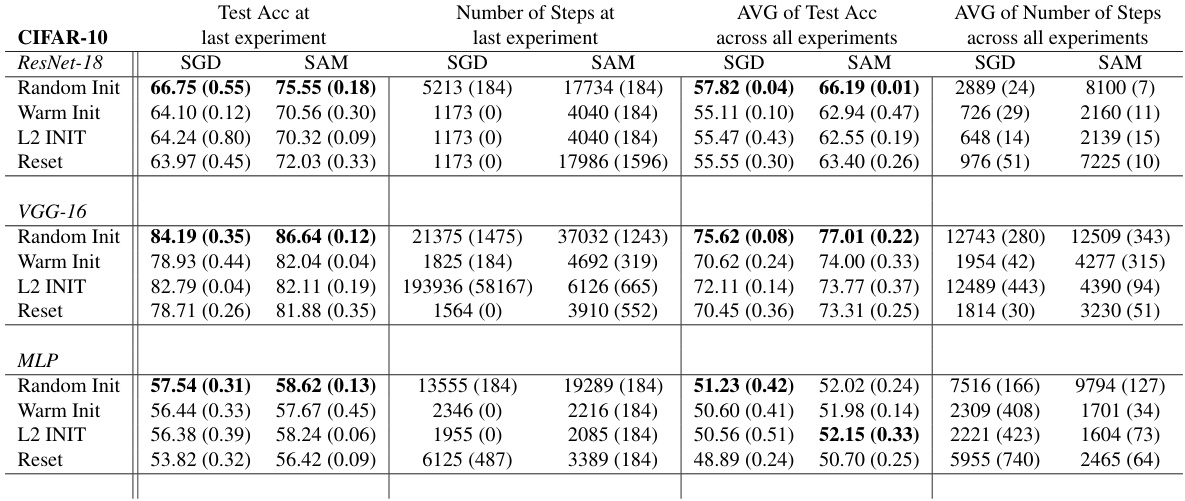
This table presents a performance comparison of different neural network training methods (Random Init, Warm Init, S&P, DASH) across four datasets (Tiny-ImageNet, CIFAR-10, CIFAR-100, SVHN) using ResNet-18. The metrics compared are test accuracy (at the last experiment and averaged across all experiments) and the number of training steps (at the last experiment and averaged across all experiments). Bold values highlight the best-performing method for each metric in each dataset. Standard deviations indicate the variability of the results.

This table presents a comparison of different neural network training methods (Random Init, Warm Init, Warm ReM, S&P, DASH) across four datasets (Tiny-ImageNet, CIFAR-10, CIFAR-100, SVHN) using ResNet-18. For each method and dataset, the table shows the test accuracy achieved at the last experiment and the average test accuracy across all experiments. It also includes the number of training steps used in the last experiment and the average number of steps across all experiments. Bold values highlight the best performing method for each metric.
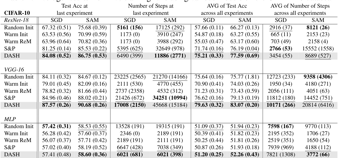
This table presents a comparison of different neural network training methods (Random Init, Warm Init, Warm ReM, S&P, and DASH) on various datasets (Tiny-ImageNet, CIFAR-10, CIFAR-100, and SVHN) using ResNet-18. The metrics reported include test accuracy at the last experiment and average across all experiments, as well as the number of training steps taken (at last experiment and average). Bold values highlight the best-performing method for each dataset and metric. The table shows that DASH generally outperforms other methods in terms of test accuracy, although sometimes at the cost of additional training steps.
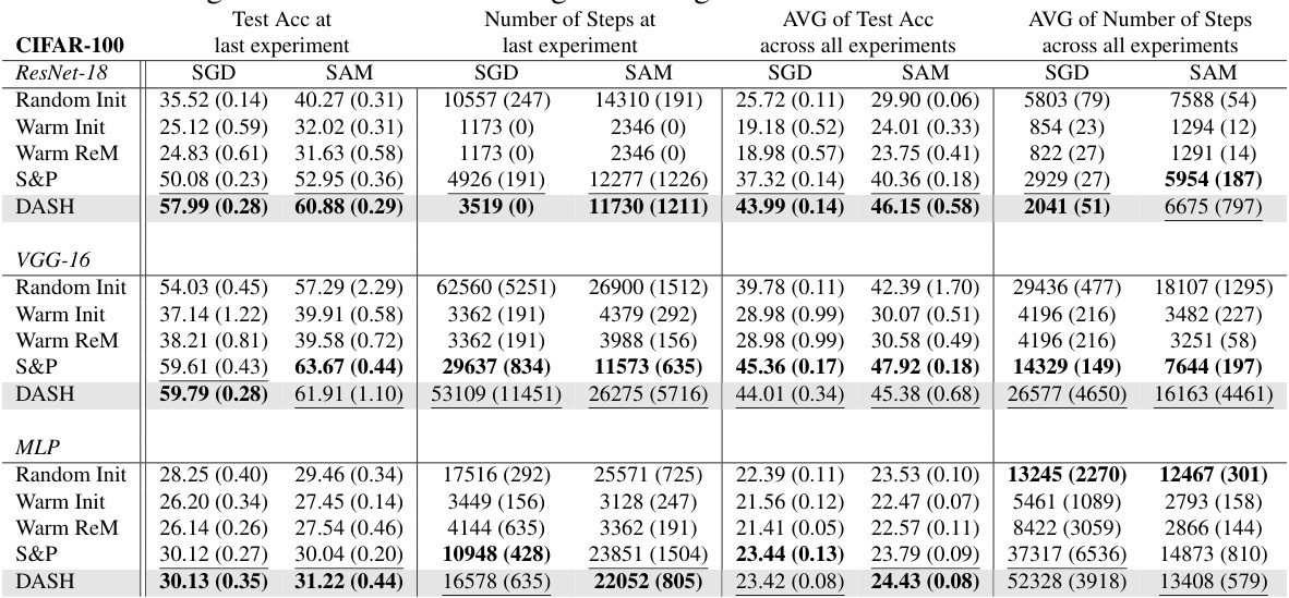
This table presents a comparison of different neural network training methods (Random Init, Warm Init, Warm ReM, S&P, DASH) on four datasets (Tiny-ImageNet, CIFAR-10, CIFAR-100, SVHN) using ResNet-18. For each dataset and method, it shows the test accuracy achieved at the last experiment, the average test accuracy across all experiments, the number of steps taken at the last experiment, and the average number of steps across all experiments. Bold values indicate the best performance in each category. The table highlights the superior performance of the DASH method in most cases, achieving higher test accuracy while often requiring fewer steps to converge.

This table presents a comparison of different neural network training methods (Random Init, Warm Init, Warm ReM, S&P, DASH) on four datasets (Tiny-ImageNet, CIFAR-10, CIFAR-100, SVHN) using ResNet-18. The table shows the test accuracy achieved at the last experiment and the average test accuracy across all experiments, along with the number of training steps for the last and average across all experiments. Bold values highlight the best-performing method for each metric. The results demonstrate the impact of different warm-starting strategies on model performance.
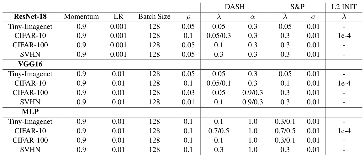
This table presents a comparison of different neural network training methods on various datasets using ResNet-18. The methods compared include random initialization (cold-starting), warm-starting, Shrink & Perturb (S&P), and the proposed DASH method. The table shows the test accuracy achieved at the last experiment and the average test accuracy across all experiments. Additionally, it reports the number of steps (training iterations) required at the last experiment and the average across all experiments. Bold values highlight the best performing method for each metric. Note that the number of random seeds used for averaging varies between datasets.
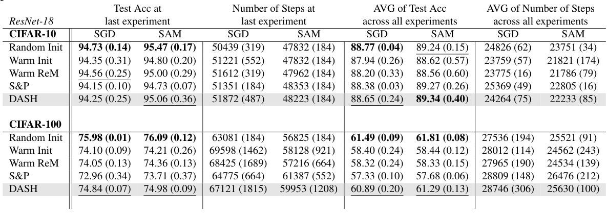
This table presents a comparison of different neural network training methods (Random Init, Warm Init, Warm ReM, S&P, DASH) on four datasets (Tiny-ImageNet, CIFAR-10, CIFAR-100, SVHN) using ResNet-18. For each dataset and method, it shows the test accuracy achieved at the last experiment, the average test accuracy across all experiments, the number of steps taken in the last experiment, and the average number of steps across all experiments. Bold values highlight the best performance for each metric. The number of random seeds used in averaging the results is also specified.

This table compares the computational and memory resources used by four different neural network training initialization methods (Cold Init, Warm Init, S&P, and DASH) on the CIFAR-10 dataset using ResNet-18. The metrics reported include the number of epochs required for training, the total training time in seconds, the total computational cost in TeraFLOPs, and the CPU and CUDA memory usage in gigabytes. The table provides insights into the efficiency and resource demands of different warm-starting strategies.

This table compares the performance of different neural network training methods (Random Init, Warm Init, S&P, and DASH) across four datasets (Tiny-ImageNet, CIFAR-10, CIFAR-100, and SVHN) using ResNet-18. For each dataset and method, it shows the test accuracy achieved at the last experiment and the average test accuracy across all experiments. It also presents the number of steps (training iterations) taken in the last experiment and the average number of steps across all experiments. Bold values highlight the best performance for each metric, except for the number of steps where bold formatting is only used for all methods except for warm-starting. Standard deviations are included to show variability across multiple runs.
Full paper#
