Causal Effect Identification in a Sub-Population with Latent Variables

↗ OpenReview ↗ NeurIPS Homepage ↗ Chat

TL;DR

#

Key Takeaways

#

Why does it matter?

#

This paper is crucial because it tackles the significant challenge of causal effect identification in sub-populations with latent variables, a common issue across various fields. The proposed algorithm and theoretical framework directly address limitations in existing causal inference methods, providing a more robust and accurate approach. This work opens up new avenues for research into causal inference problems in complex settings and has implications for a wide range of applications where sub-population analysis is critical.

Visual Insights

#

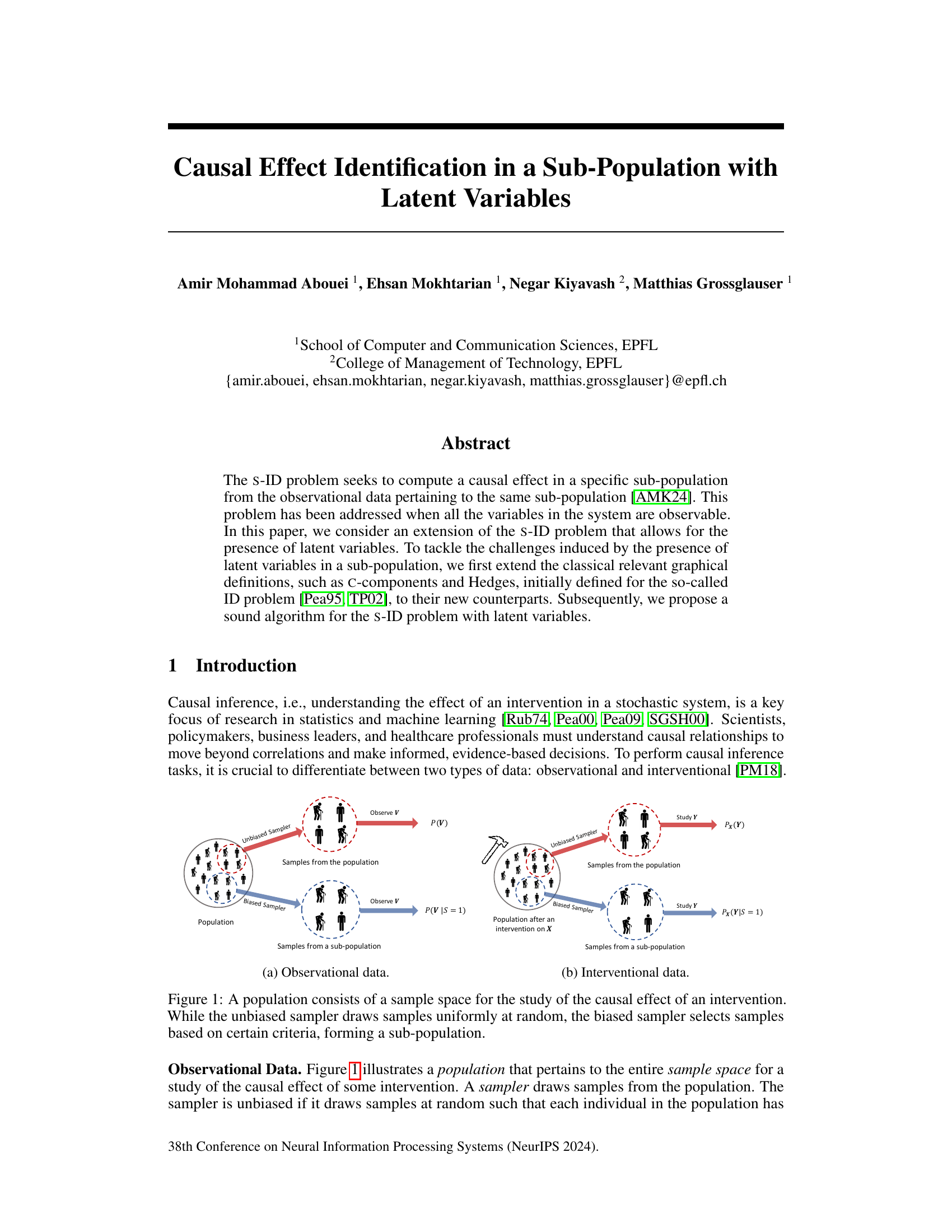
This figure illustrates two types of data used in causal inference: observational and interventional data. Observational data is collected from an unbiased sampler, drawing samples uniformly from the entire population and providing the distribution P(V). Interventional data involves an intervention on a subset of variables (X) and then observing the effect on other variables (Y) in the population; an unbiased sampler would then give the distribution P_x(Y). The figure also shows how a biased sampler selects a sub-population based on criteria (S=1) resulting in conditional distributions P(V|S=1) for observational data and P_x(Y|S=1) for interventional data. These sub-population distributions are the central focus of the s-ID problem.

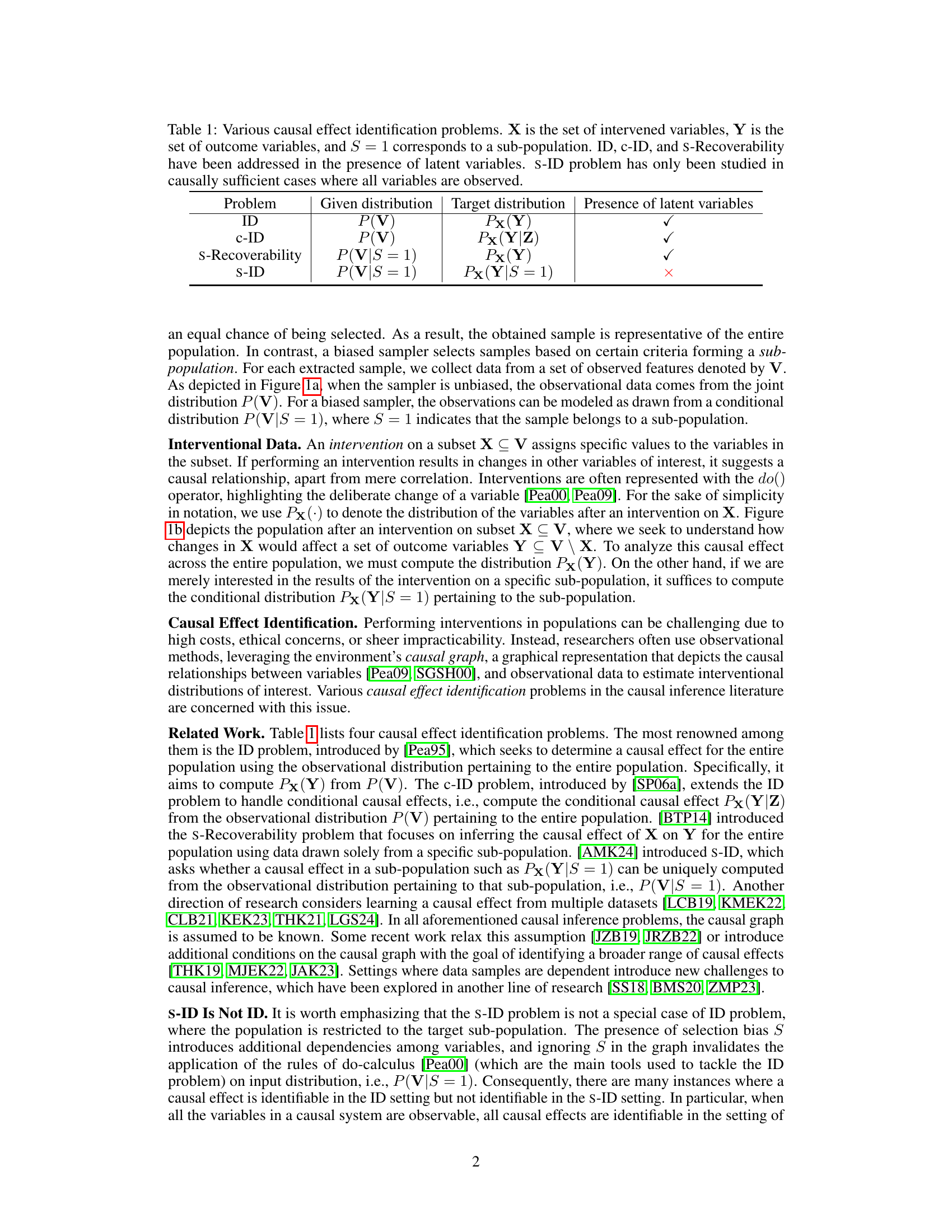
This table compares four causal effect identification problems: ID, c-ID, s-Recoverability, and S-ID. It shows the given and target distributions for each problem, and indicates whether latent variables are considered. The ID problem identifies causal effects for the entire population; c-ID extends this to conditional causal effects; s-Recoverability focuses on inferring causal effects from a sub-population for the entire population; and the S-ID problem focuses on uniquely identifying a causal effect within a specific sub-population.

In-depth insights

#

S-ID with Latent Variables

#

The subheading “S-ID with Latent Variables” suggests an extension of the standard S-ID (Subpopulation-identifiable causal effect) problem to scenarios involving unobserved variables. The core challenge lies in identifying causal effects within a specific subpopulation when some variables are latent, making traditional causal inference methods inadequate. This necessitates new theoretical frameworks and algorithms that can handle the added complexity of latent variables. The approach likely involves extending existing graphical criteria (like c-components and hedges) used in causal discovery to account for the presence of latent variables within the subpopulation context. This extension likely requires careful modification of existing definitions to ensure compatibility with subpopulation analysis while accounting for the impact of unobserved confounders or mediators. The proposed solution would probably involve a novel algorithm designed to identify and handle these latent variables effectively, possibly incorporating techniques from latent variable modeling or graphical causal inference with latent variables. Ultimately, the goal is to develop a method that reliably identifies causal effects within a specific subpopulation even in the presence of latent variables, a significant advancement in causal inference methods.

Graphical Criteria for s-ID

#

Developing graphical criteria for identifying causal effects within subpopulations (s-ID) presents a significant challenge. Existing methods often rely on simplifying assumptions, such as the absence of latent variables or selection bias. A robust approach must account for the complexities introduced by these factors, which can obscure causal relationships and lead to misidentification. A key aspect is extending existing graphical concepts (like c-components and hedges used in the ID problem) to handle latent variables and subpopulation selection. This involves carefully defining new graphical structures that capture the conditional dependencies and ensure correct identification. Sufficient graphical criteria are necessary to determine when a causal effect is identifiable, but also efficient algorithms are required to compute the effect once identifiability is established. The development of such criteria and algorithms will be a crucial step in advancing causal inference in real-world settings with complex data structures and unobserved variables.

Algorithm for S-ID

#

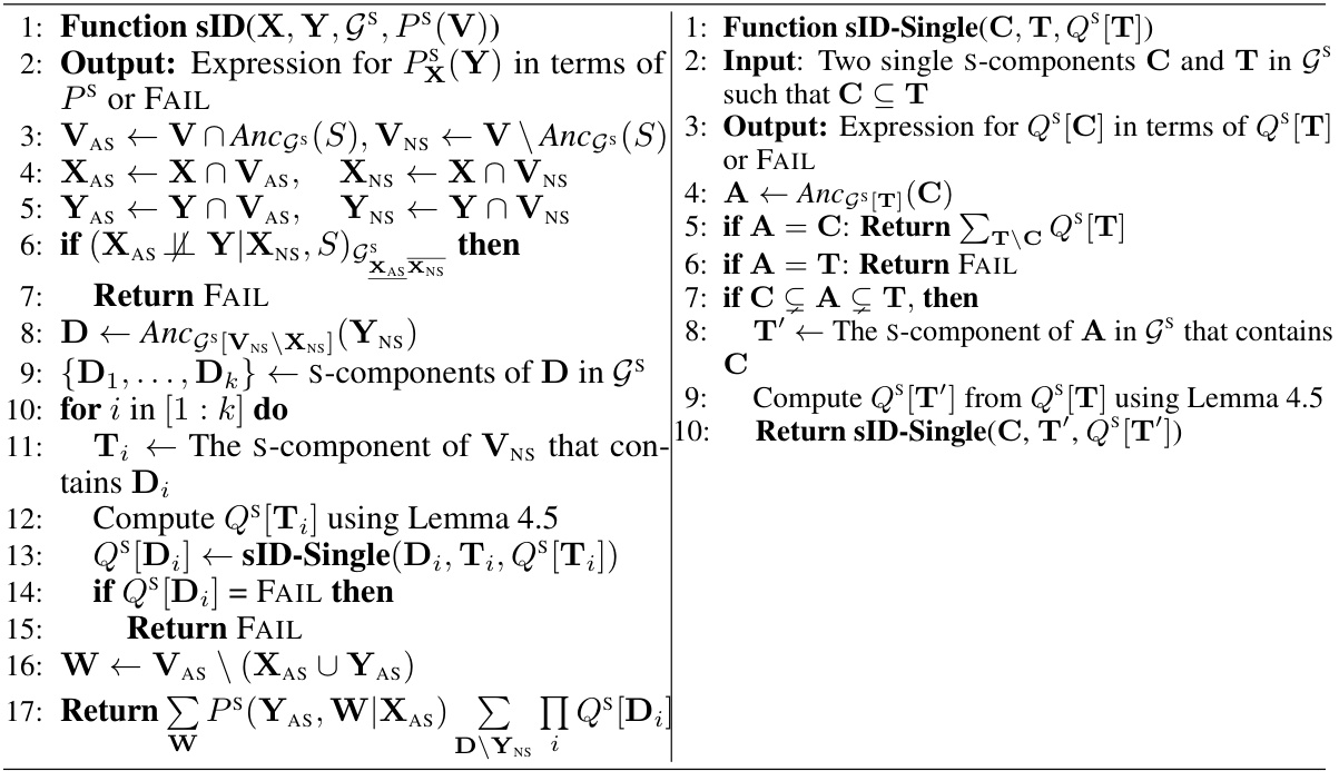
The section ‘Algorithm for S-ID’ would detail a computational procedure to determine if a causal effect is identifiable within a subpopulation (S-ID), particularly when latent variables are present. The algorithm’s design would likely leverage the extended graphical criteria (c-components and Hedges) adapted for the S-ID problem. It would recursively check for the presence of s-Hedges in the augmented causal graph, a modified concept to handle latent variables and selection bias. A crucial aspect would be the algorithm’s soundness, meaning it only identifies truly identifiable effects, avoiding false positives. The algorithm’s inputs would include the augmented ADMG, the observational distribution conditioned on the subpopulation, and sets X and Y representing the intervention and outcome variables. The output would be either a formula expressing the causal effect in terms of the input distribution or a ‘FAIL’ if identifiability is not guaranteed. The complexity of the algorithm stems from managing latent variables and selection bias, requiring careful manipulation of conditional probabilities. This necessitates the development of efficient methods for calculating conditional distributions within the subpopulation, potentially utilizing advanced graphical model techniques. The algorithm’s efficiency and scalability would also be significant considerations, especially for large-scale datasets.

S-Recoverability Reduction

#

The concept of ‘S-Recoverability Reduction’ in causal inference tackles the challenge of identifying causal effects within a subpopulation using only observational data from that subpopulation. A key insight is the relationship between S-recoverability and the broader S-ID problem. S-recoverability focuses on identifying the causal effect of an intervention on a specific outcome variable within a biased sample. Showing a reduction from S-recoverability to S-ID implies that solving the more general S-ID problem also solves the S-recoverability problem. This is significant because it simplifies the task and reduces computational complexity. However, the reduction may not always be straightforward. The conditions under which such a reduction holds need careful consideration, potentially involving restrictions on the causal structure and conditional independencies among variables in the subpopulation. Future work could explore relaxing these conditions to broaden the applicability of this reduction and potentially developing more efficient algorithms for causal effect identification under selection bias.

Limitations and Future Work

#

A thoughtful consideration of limitations and future work in the context of causal effect identification within sub-populations, especially when dealing with latent variables, should acknowledge the algorithmic assumptions that might restrict applicability. Extending the algorithm’s capabilities to handle more complex causal structures and addressing scalability challenges for large datasets would be beneficial. Future research could explore relaxing assumptions regarding the observational data’s faithfulness to the underlying causal model and how to incorporate various forms of prior knowledge or domain expertise. Investigating the sensitivity of the method to model misspecification and exploring techniques for uncertainty quantification would greatly enhance practical utility. Finally, investigating the interplay between latent variables and selection bias to provide more robust identification strategies warrants further study.

More visual insights

#

More on figures

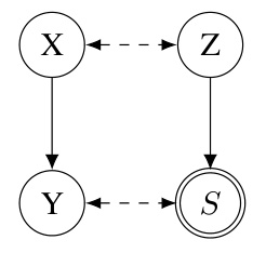
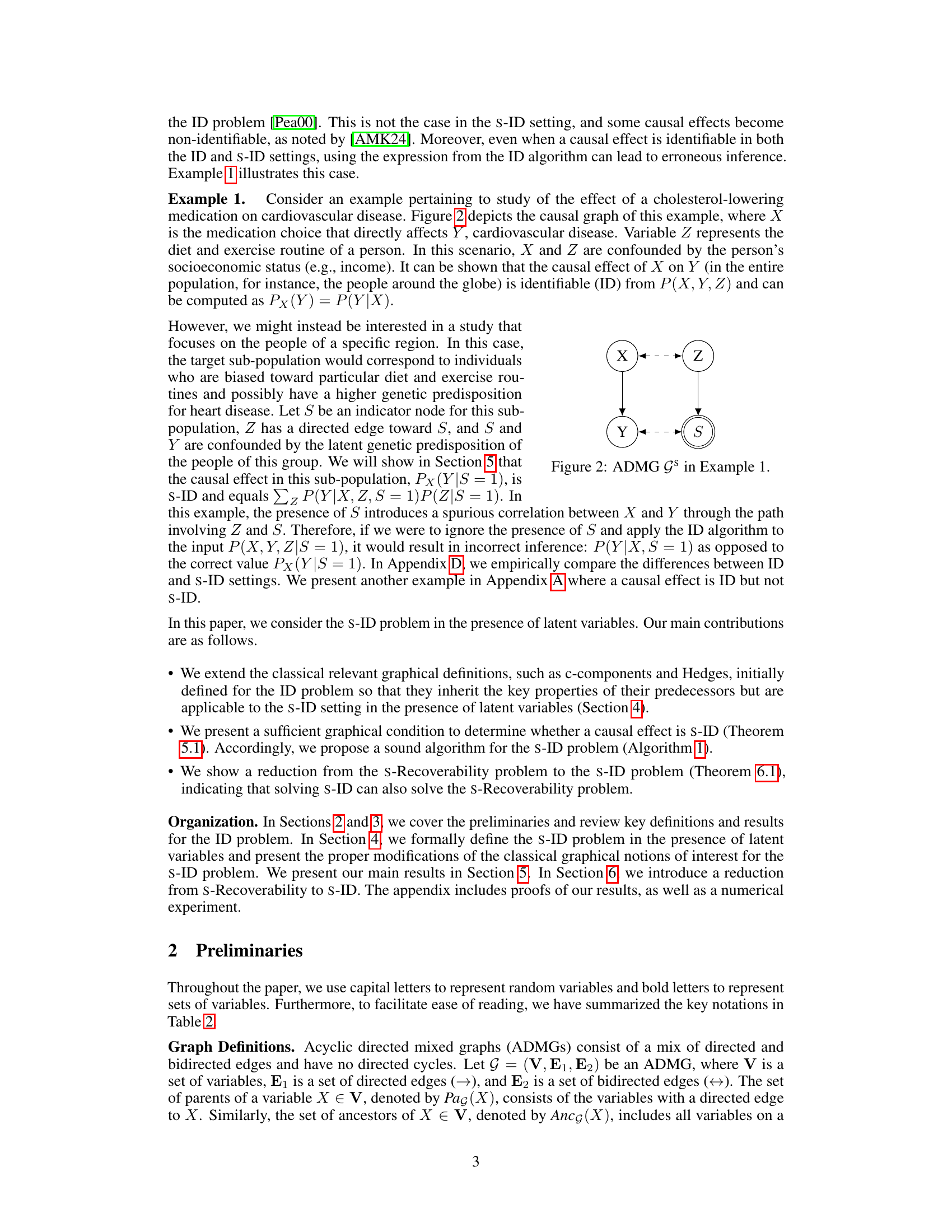
This ADMG represents the causal relationships between variables in Example 1 of the paper, which discusses the effect of a cholesterol-lowering medication (X) on cardiovascular disease (Y), considering diet and exercise (Z) as a confounder and socioeconomic status as a latent variable influencing both the medication choice and the diet/exercise habits (S). The directed edges show direct causal effects, while the bidirected edge represents confounding between X and Z due to the latent variable, which further affects the subpopulation indicator (S). The figure visually illustrates the complexities of causal inference in the presence of latent variables and selection bias within a specific sub-population.

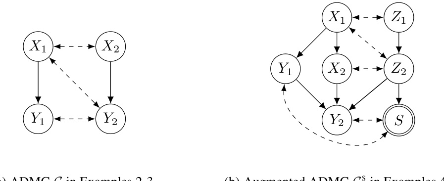
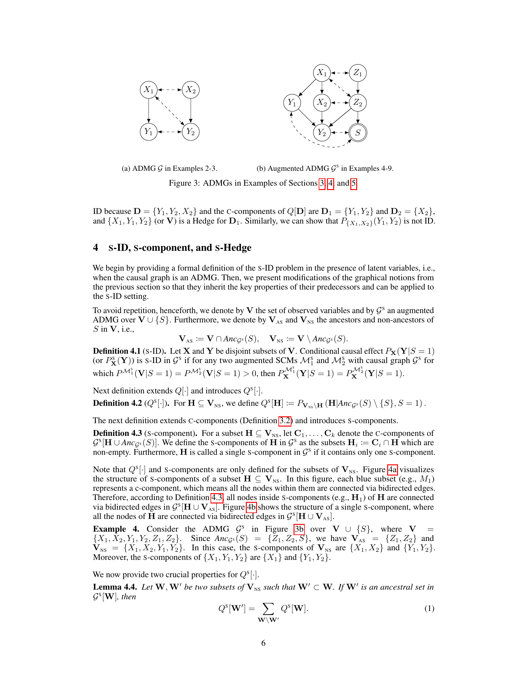
This figure contains two ADMGs (Acyclic Directed Mixed Graphs). (a) shows an ADMG used in examples 2 and 3 in the paper to illustrate the concept of C-components and Hedges. (b) is an augmented ADMG (including an auxiliary variable S representing sub-population) used in examples 4 and 5 to illustrate the concept of s-components and s-Hedges. Both figures are essential for understanding the theoretical concepts of causal effect identification in the paper, particularly how the introduction of a sub-population (represented by S) affects the graphical structures and identification methods.

This figure visualizes several graph structures relevant to the concepts of s-components and s-hedges introduced in the paper. Panel (a) shows the s-components of a set H, which are subsets of H that are connected via bidirected edges in a subgraph. Panel (b) illustrates the case where H is a single s-component. Panel (c) depicts an s-Hedge for Y (a single s-component), satisfying certain conditions on its ancestors and connectivity. Finally, panel (d) shows a Hedge for Y, which is a simplified case of an s-Hedge that does not include the auxiliary variable S used to define sub-populations.

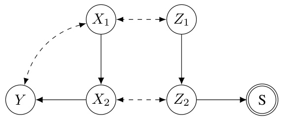
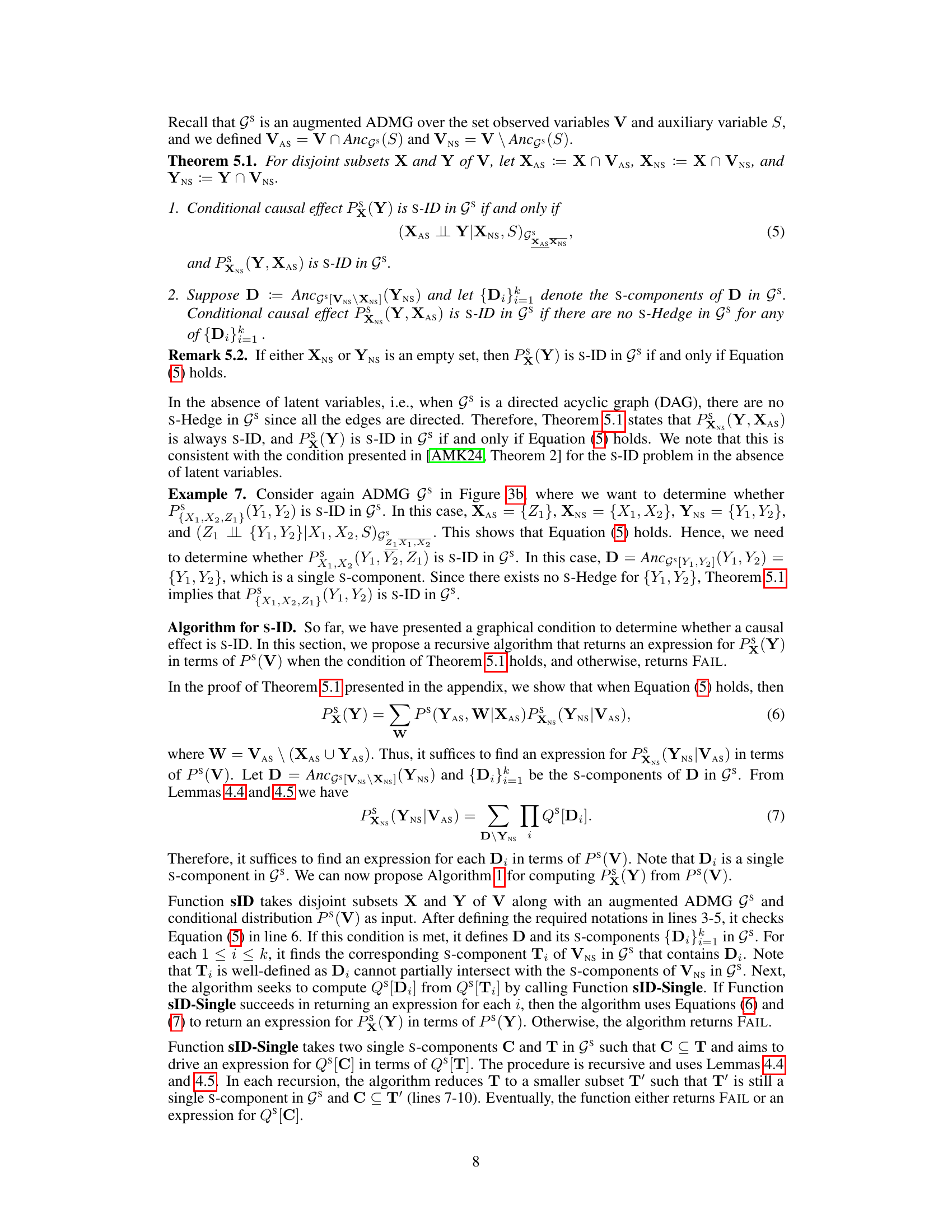
This figure shows two ADMGs (Acyclic Directed Mixed Graphs). Figure 3a depicts an ADMG used in examples illustrating concepts like C-components and Hedges in Section 3, which focuses on the ID problem (identifiability of causal effects in the full population). Figure 3b is an augmented ADMG that includes an auxiliary variable ‘S’ representing a sub-population. This augmented ADMG is used in the examples of Sections 4 and 5 which extend the ID problem to the S-ID problem (identifiability in a specific subpopulation). The addition of ‘S’ is crucial to the S-ID problem, highlighting the different challenges in identifying causal effects within a subpopulation compared to the full population.

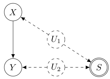
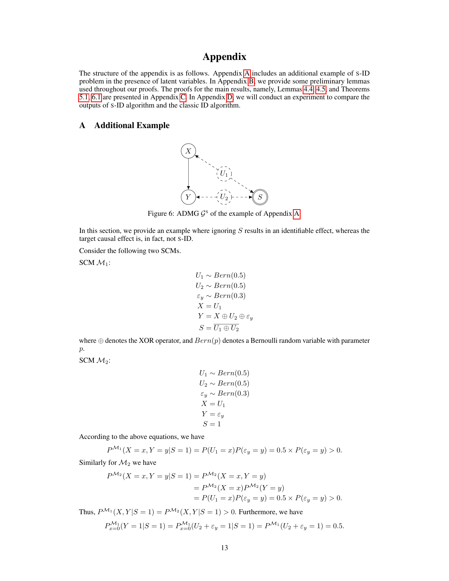
This ADMG shows the causal relationships between variables X, Y, and S, with latent variables U1 and U2. X is a direct cause of Y. U1 affects both X and S, indicating a confounding relationship between X and S. U2 affects both Y and S, showing a confounding effect between Y and S. The dashed lines represent bidirected edges indicating latent confounders. The circle around S denotes it as an indicator of sub-population selection bias.

This ADMG shows the causal relationships between variables X, Y, and S, with latent variables U1 and U2 representing unobserved confounders. It illustrates an example where a causal effect is identifiable in the full population (ID) but not identifiable in a specific sub-population (not s-ID), even though there is no selection bias present in the observed variables.

More on tables

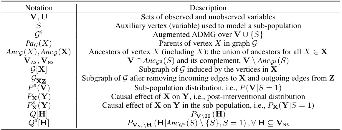
This table compares four causal effect identification problems: ID, c-ID, s-Recoverability, and S-ID. It shows the given distribution, target distribution, and whether latent variables are considered for each problem. The table highlights that the S-ID problem has only been studied in cases where all variables are observed (causally sufficient), while the others have been studied in the presence of latent variables.

This table compares four causal effect identification problems: ID, c-ID, s-Recoverability, and S-ID. It shows the given distribution, target distribution, and whether latent variables are considered for each problem. The table highlights that the S-ID problem, the focus of the paper, has only been studied previously when all variables are observable (causally sufficient).

Full paper

#