↗ OpenReview ↗ NeurIPS Homepage ↗ Chat
TL;DR#
Training deep neural networks often involves optimizing their parameters to achieve better generalization performance. A recent optimization method called Sharpness-Aware Minimization (SAM) has shown promise in enhancing generalization, but it suffers from high computational costs due to sequential gradient calculations. This slows down the training process and limits its applicability.
The paper introduces SAMPa, a novel modification of SAM that addresses its limitations. By cleverly parallelizing the two gradient computations required in SAM, SAMPa accelerates the training process without sacrificing generalization performance. In fact, it consistently outperforms SAM across various machine learning tasks. The authors also provide theoretical guarantees for convergence, even when using a fixed perturbation size which is a notable improvement over existing methods. These improvements make SAMPa a more practical and effective optimization technique for training deep learning models.
Key Takeaways#
Why does it matter?#
This paper is crucial for researchers working on optimization algorithms for deep neural networks. It presents SAMPa, a significantly improved version of the sharpness-aware minimization (SAM) technique, offering substantial speedup and improved generalization. This advancement directly addresses a critical limitation of SAM, its high computational cost, while maintaining or even improving its performance. The proposed method and accompanying theoretical analysis offer valuable insights and open avenues for developing more efficient SAM-based methods. Its impact extends across various applications requiring improved DNN generalization, from computer vision to natural language processing.
Visual Insights#
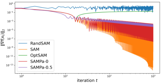
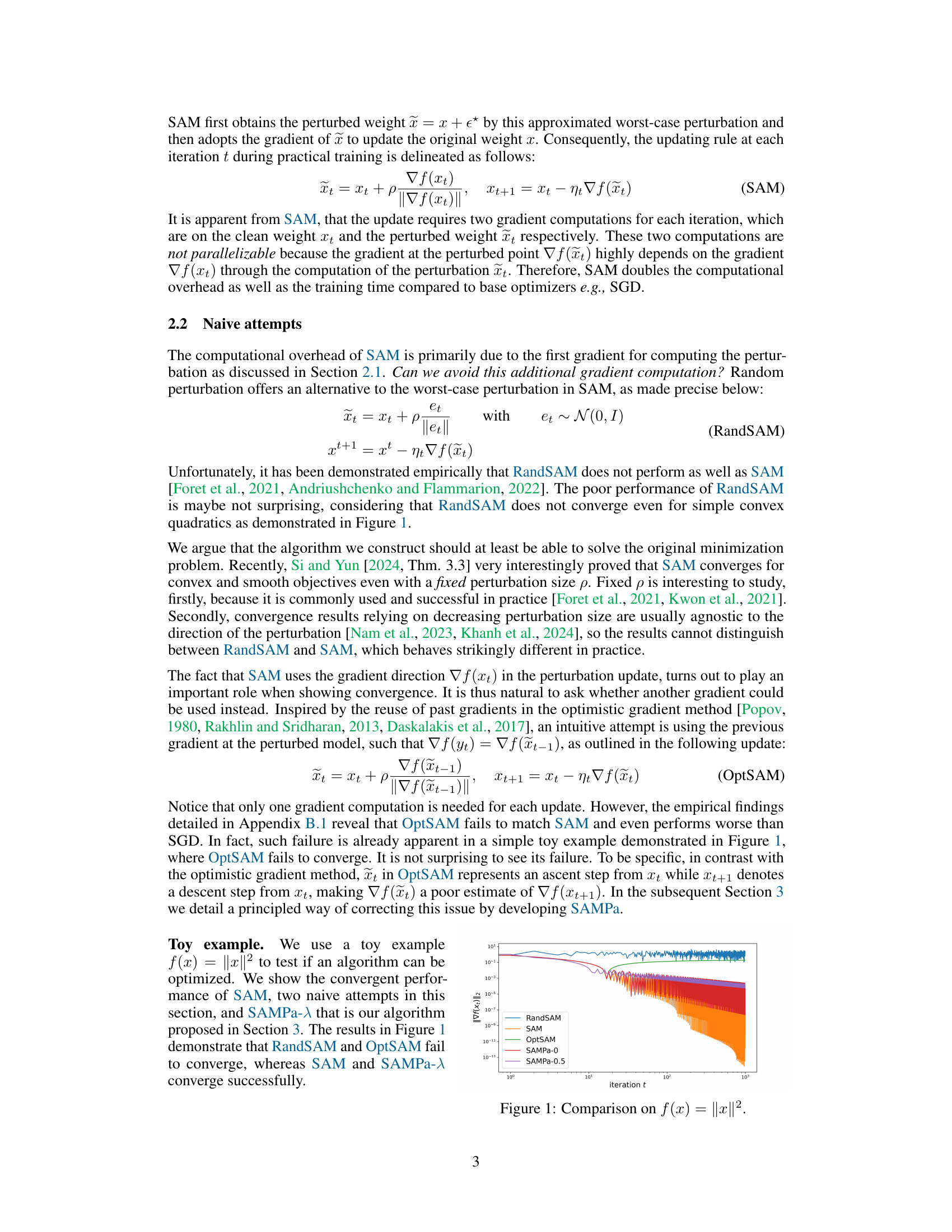
This figure compares the convergence performance of different algorithms on a simple convex quadratic function f(x) = ||x||². It demonstrates that RandSAM and OptSAM, two naive attempts at parallelizing SAM, fail to converge, highlighting the challenges involved in parallelizing the SAM algorithm. In contrast, SAM and SAMPa-λ (a variant of SAMPa with λ=0 and λ=0.5) converge successfully, showcasing the effectiveness of the proposed parallelization approach. The y-axis represents the squared norm of the gradient (||∇f(x)||²), indicating the proximity to a minimum. The x-axis represents the number of iterations.

This table presents the test accuracies achieved by different models (DenseNet-121, Resnet-56, VGG19-BN, WRN-28-2, WRN-28-10) on the CIFAR-10 dataset using various optimization methods: SGD, SAM, SAMPa-0, SAMPa-0.2 (with 200 epochs), and SAMPa-0.2 (with 400 epochs). The ‘Temporal cost’ column indicates the number of gradient computations per epoch, showcasing the efficiency gains of SAMPa. The results demonstrate that SAMPa-0.2 achieves higher accuracy than SAM while using only half the computational cost (or the same cost when comparing 400 epochs).
In-depth insights#
SAMPa: Parallel SAM#
The proposed method, SAMPa, tackles the computational inefficiency of Sharpness-Aware Minimization (SAM) by enabling the parallelization of its two gradient computations. This is a significant improvement as SAM’s sequential nature doubles the computational cost compared to standard optimizers. SAMPa achieves a twofold speedup under ideal conditions (negligible communication overhead). Empirical results demonstrate that SAMPa is highly efficient and consistently outperforms the original SAM across vision and language tasks. A key theoretical contribution lies in proving convergence guarantees for SAMPa even with fixed perturbation sizes, achieved through a novel Lyapunov function. This theoretical foundation makes SAMPa a robust and reliable alternative. The parallelization strategy in SAMPa is not trivial; it requires a novel optimization sequence to break the inherent sequential dependency in SAM’s original formulation. The success of this approach suggests that designing parallel variants of SAM-based methods can be effectively guided by the requirement of maintaining strong convergence guarantees.
Convergence Analysis#
A rigorous convergence analysis is crucial for establishing the reliability and trustworthiness of any optimization algorithm. In the context of a sharpness-aware minimization algorithm, a convergence analysis would demonstrate, under specific assumptions (like convexity and Lipschitz continuity of the loss function), that the algorithm’s iterates indeed approach a solution that minimizes the sharpness of the loss landscape. A key aspect would be proving that a suitably chosen Lyapunov function decreases monotonically across iterations. Establishing convergence guarantees, especially for fixed perturbation sizes, which is often not straightforward, would be a significant theoretical contribution. The analysis may involve techniques from optimization theory, such as gradient descent analysis, and might incorporate specific properties of the sharpness-aware approach, resulting in convergence rates (e.g., sublinear or linear) under various conditions. Furthermore, the analysis could investigate how factors like the perturbation size and step size influence the convergence behavior. A complete analysis would ideally consider both theoretical convergence properties and practical implications, relating them to the algorithm’s generalization performance. A tight analysis would go beyond merely proving convergence and shed light on the rate of convergence, offering insights into the algorithm’s efficiency and helping to guide the selection of hyperparameters in practice.
Efficiency Gains#
The research paper highlights significant efficiency gains achieved by the proposed SAMPa algorithm compared to the original SAM method. This improvement stems from the parallelization of gradient computations, a key computational bottleneck in SAM. By cleverly restructuring the algorithm, SAMPa enables simultaneous calculation of the two gradients required by SAM, leading to a two-fold speedup. Theoretical analysis confirms the convergence of SAMPa, even with fixed perturbation sizes. Empirical results demonstrate that SAMPa consistently outperforms SAM across various tasks, further highlighting the practical benefits of this optimization technique. The reduced computational cost makes SAMPa a more efficient and attractive choice for training large and complex neural networks, leading to significant improvements in training time and resources. While other efficient SAM variants exist, SAMPa’s combination of theoretical guarantees and demonstrated practical speedups positions it as a powerful tool for improving the efficiency of sharpness-aware minimization.
Broader Impacts#
The research paper’s core contribution is an efficient optimization algorithm, SAMPa, enhancing the performance of existing sharpness-aware minimization methods. Its broader impact is primarily methodological, improving the efficiency and generalization capabilities of deep learning models across various domains (vision, language). While the paper doesn’t directly address societal impacts, its implications are significant. Improved efficiency translates to reduced energy consumption and computational costs during model training, thus promoting environmentally friendly AI development. Enhanced generalization can lead to more reliable and robust AI systems in various applications, potentially benefitting numerous sectors such as healthcare and autonomous driving. However, potential risks exist. The increased efficiency could lower the barrier to entry for malicious actors seeking to develop harmful AI applications. The paper acknowledges this but does not delve into specific mitigation strategies, leaving that area open for future research and ethical considerations. Therefore, future work needs to focus on exploring both the beneficial and detrimental consequences of SAMPa’s widespread adoption.
Future of SAMPa#
The future of SAMPa hinges on addressing its current limitations and exploring new avenues for improvement. Further theoretical analysis is crucial to understand its convergence properties beyond convex settings and to potentially adapt it to non-smooth or non-convex loss landscapes. Investigating the impact of varying perturbation sizes and exploring adaptive strategies for choosing the optimal perturbation could significantly enhance SAMPa’s performance and robustness. Exploring efficient parallel implementations on diverse hardware architectures, beyond the current two-GPU setup, is essential to maximize its scalability and make it accessible to a broader range of users. Additionally, research into alternative methods for calculating gradients in parallel could yield improvements in computational efficiency and accuracy. Finally, integrating SAMPa with other optimization techniques and exploring its application in diverse domains beyond image classification and NLP, such as reinforcement learning, will expand its impact and reveal new possibilities.
More visual insights#
More on figures
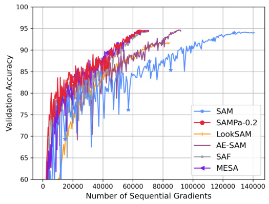
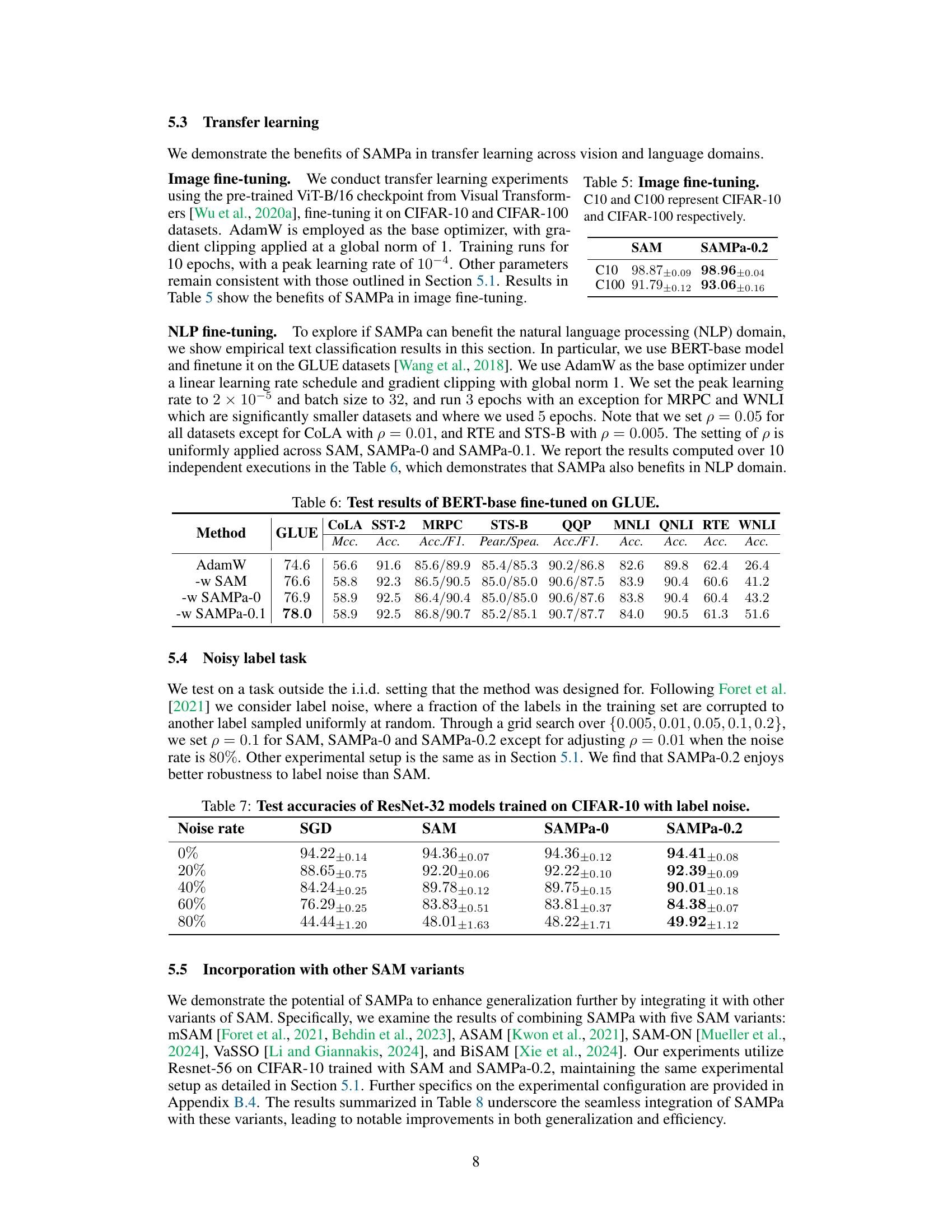
This figure compares the computational time of different efficient variants of the Sharpness-Aware Minimization (SAM) algorithm. The x-axis represents the number of sequential gradient computations, reflecting the computational cost in an idealized scenario. The y-axis shows the actual runtime in seconds. The figure demonstrates that SAMPa-0.2 achieves the shortest runtime, significantly outperforming other methods such as LookSAM, AE-SAM, SAF, MESA, and ESAM, both in terms of the number of sequential gradient computations and in actual wall-clock time. This highlights the efficiency of SAMPa-0.2 in practical settings.

This figure compares the computational time of various efficient SAM (Sharpness-Aware Minimization) variants. The top panel (a) shows the number of sequential gradient computations, a theoretical measure of efficiency. The bottom panel (b) displays the actual training time in seconds, which incorporates factors like forward/backward passes and communication overhead. SAMPa-0.2 consistently shows a significantly reduced computational time compared to other methods, achieving near-minimal runtime in both theoretical and practical settings.

This figure compares the computational time of several efficient SAM variants. The left subplot (a) shows the number of sequential gradient computations, a theoretical measure of computational cost. The right subplot (b) depicts the actual wall-clock training time. SAMPa-0.2 consistently demonstrates the lowest computational time, both theoretically and practically, outperforming other efficient SAM variants, highlighting its efficiency gains.
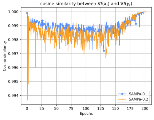
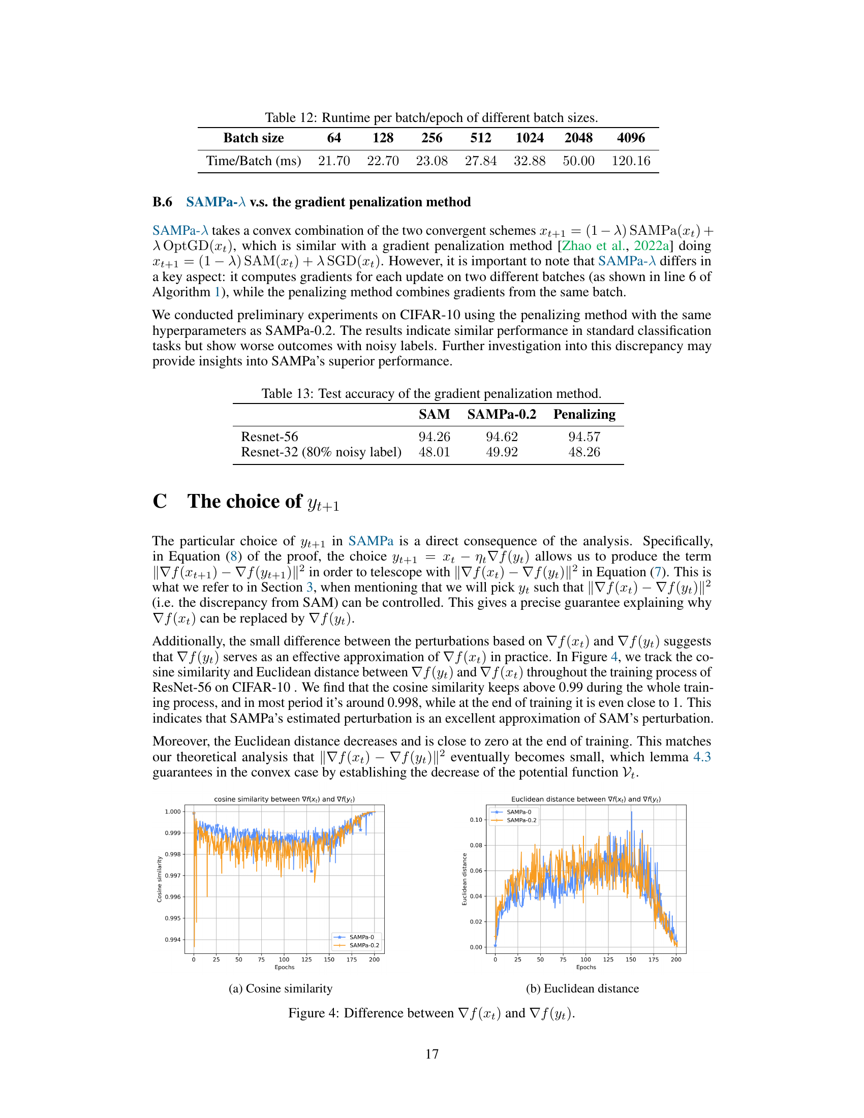
This figure shows the cosine similarity and Euclidean distance between the gradients ∇f(xt) and ∇f(yt) throughout the training process of ResNet-56 on CIFAR-10. The cosine similarity remains consistently high (above 0.99), indicating a close approximation between the gradients. The Euclidean distance decreases over time and approaches zero at the end of training, further demonstrating the effectiveness of the approximation used in SAMPa.
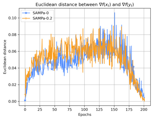
This figure shows the cosine similarity and Euclidean distance between the gradients ∇f(xt) and ∇f(yt) during the training process of ResNet-56 on CIFAR-10. The cosine similarity remains consistently high (above 0.99), indicating that the gradients are very similar. The Euclidean distance decreases over epochs, approaching zero at the end of training. This visual representation supports the claim that ∇f(yt) serves as a good approximation for ∇f(xt) in SAMPa, which is crucial for the algorithm’s parallelization and convergence.
More on tables

This table presents the test accuracies achieved by different models (DenseNet-121, Resnet-56, VGG19-BN, WRN-28-2, WRN-28-10) on the CIFAR-100 dataset using various optimization methods: SGD, SAM, SAMPa-0, SAMPa-0.2 (with 200 epochs), and SAMPa-0.2 (with 400 epochs). The ‘Temporal cost’ column indicates the number of gradient computations per update. The results highlight that SAMPa-0.2 consistently outperforms SAM while maintaining a significantly reduced computational cost (halved). The inclusion of SAMPa-0.2 with 400 epochs allows for a direct comparison with SGD and SAM, showcasing the performance gains.

This table presents the Top1 and Top5 accuracies achieved by SAM and SAMPa-0.2 on the ImageNet-1K dataset. The results demonstrate the performance of both algorithms in a large-scale image classification task. Top1 accuracy refers to the percentage of images correctly classified into their top predicted class, while Top5 accuracy represents the percentage of images correctly classified into one of their top 5 predicted classes. The values are presented as mean ± standard deviation, indicating the variability in the results across multiple independent experiments.

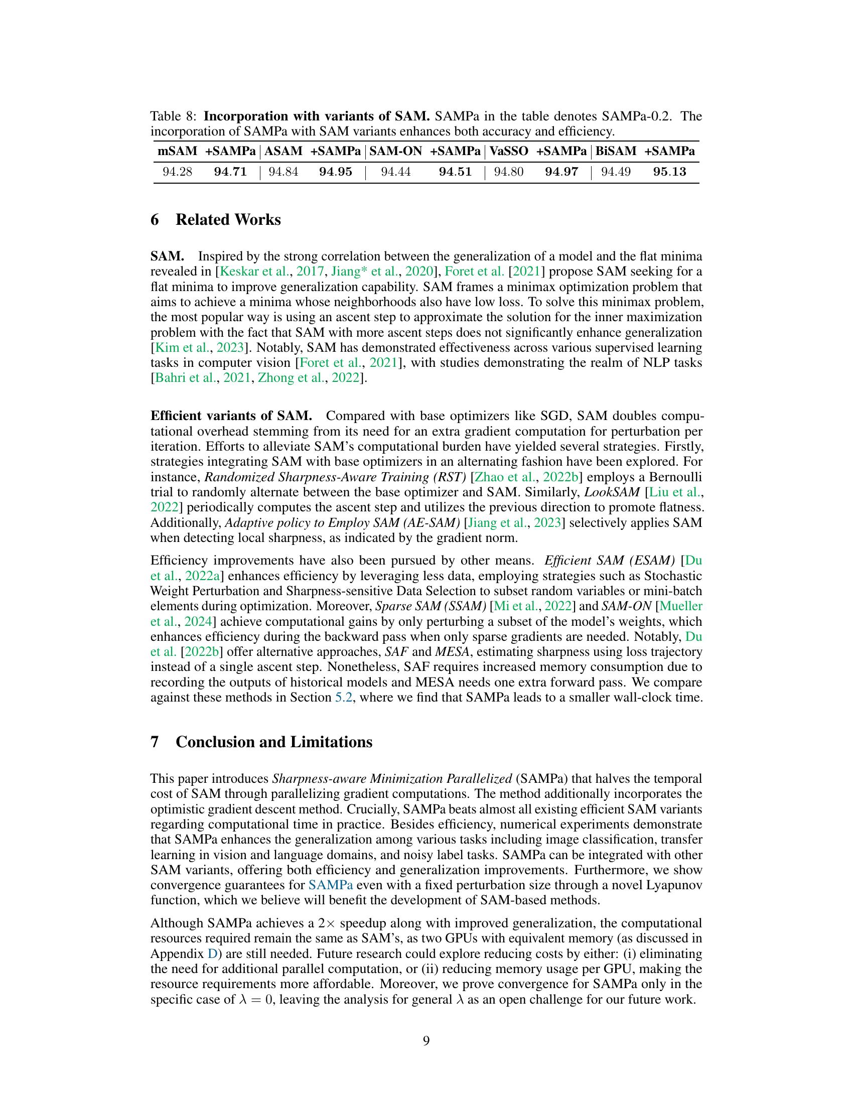
This table compares the performance of SAMPa-0.2 with several other efficient variants of the SAM algorithm. The comparison includes test accuracy and the time per epoch. The results show that SAMPa-0.2 achieves high accuracy with a significantly reduced computation time compared to other methods.

This table presents the results of image fine-tuning experiments using the pre-trained ViT-B/16 checkpoint. The model was fine-tuned on the CIFAR-10 and CIFAR-100 datasets using AdamW optimizer. The table shows the top-1 test accuracy achieved by SAM and SAMPa-0.2 on both datasets after 10 epochs of training. SAMPa-0.2 shows improved accuracy compared to SAM.

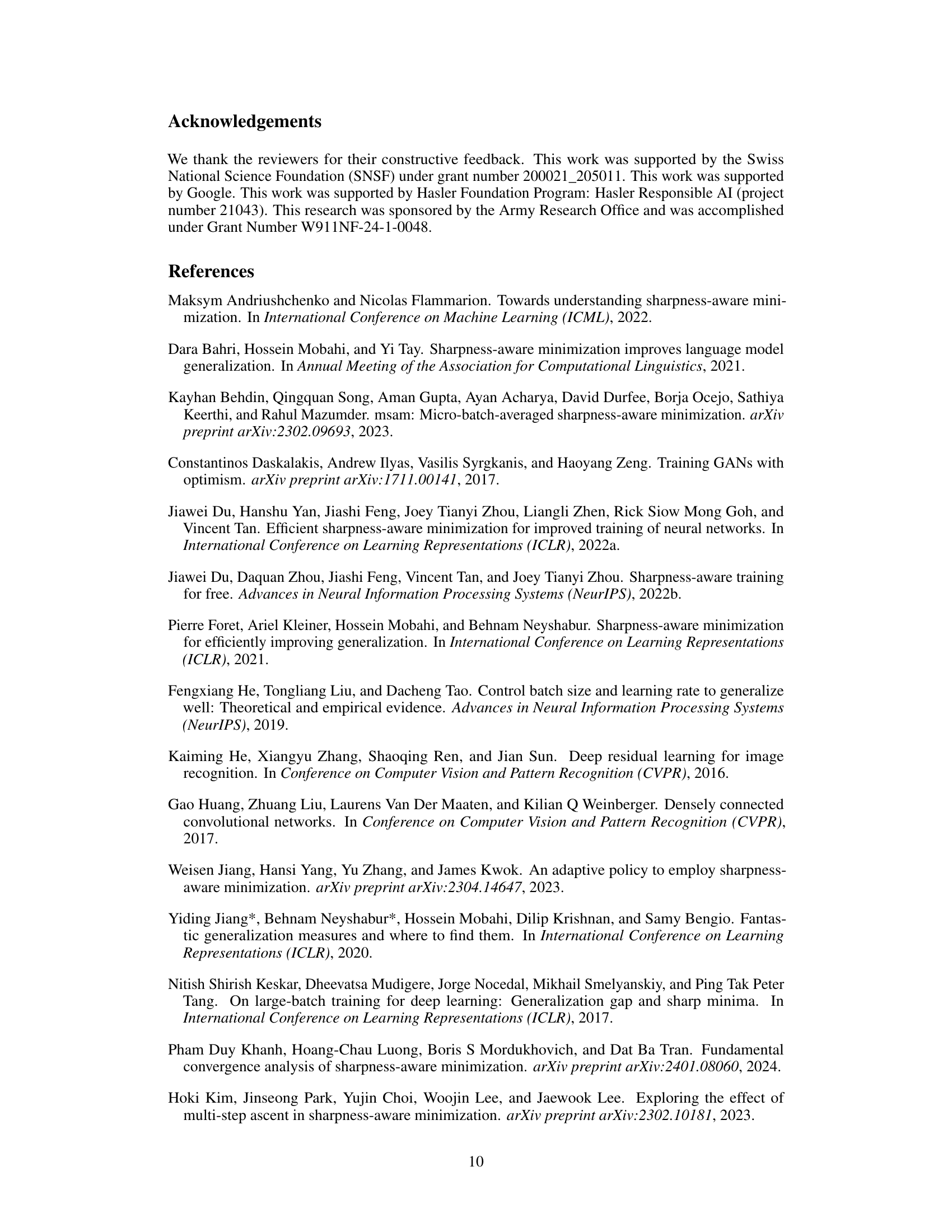
This table presents the results of fine-tuning a BERT-base model on the GLUE benchmark dataset using different optimization methods: AdamW, AdamW with SAM, AdamW with SAMPa-0, and AdamW with SAMPa-0.1. The table shows the performance metrics (accuracy, MCC, F1-score, Pearson/Spearman correlation) achieved by each method on various GLUE tasks: CoLA, SST-2, MRPC, STS-B, QQP, MNLI, QNLI, RTE, and WNLI. It demonstrates the effectiveness of SAMPa-0.1 in improving the performance of BERT-base for NLP tasks in the GLUE benchmark.

This table presents the test accuracies of ResNet-32 models trained on CIFAR-10 datasets with varying levels of label noise (0%, 20%, 40%, 60%, 80%). The results are compared across four different optimization methods: SGD, SAM, SAMPa-0, and SAMPa-0.2. Each entry represents the average test accuracy ± standard deviation obtained over multiple independent runs. The table demonstrates the robustness of SAMPa-0.2 against label noise, achieving consistently higher accuracies compared to SAM and SGD, especially at higher noise rates.

This table presents the results of integrating SAMPa with several other variants of SAM algorithms. It shows the test accuracy achieved by each combination on the CIFAR-10 dataset using the ResNet-56 model. The results demonstrate that incorporating SAMPa consistently improves the accuracy, highlighting its potential as a beneficial addition to existing SAM methods. SAMPa-0.2 is used in all combinations shown.

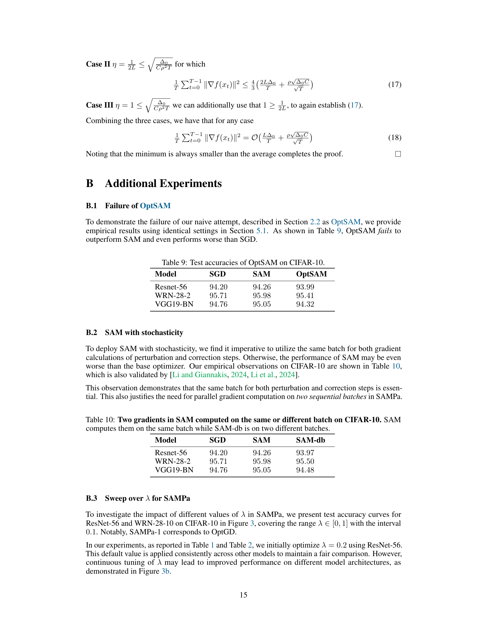
This table presents the test accuracies achieved by three different optimization methods: SGD (Stochastic Gradient Descent), SAM (Sharpness-Aware Minimization), and OptSAM (a naive attempt at parallelizing SAM) on the CIFAR-10 dataset. It demonstrates that OptSAM, a proposed alternative to SAM, performs worse than SAM and even underperforms the standard SGD, highlighting the challenges involved in naively parallelizing SAM.

This table compares the test accuracy of three different methods (SGD, SAM, and SAM-db) on the CIFAR-10 dataset using three different models (Resnet-56, WRN-28-2, and VGG19-BN). SAM-db represents a variation of SAM where the two gradient computations are performed on different batches instead of the same batch. The results show that using the same batch for both gradient computations in SAM leads to slightly better performance compared to using different batches in SAM-db, and both methods generally outperform SGD.

This table compares the performance of SAMPa-0.2 against other efficient variants of SAM on the CIFAR-10 dataset using ResNet-56. It presents the test accuracy and time per epoch for each method, highlighting the efficiency and improved generalization capabilities of SAMPa-0.2. The results show that SAMPa-0.2 achieves superior accuracy with significantly less computational time compared to most other SAM variants.

This table presents the test accuracies achieved on the CIFAR-10 dataset using various models and optimization methods. It compares the performance of SGD, SAM (Sharpness-Aware Minimization), and different variants of SAMPa (a parallelized version of SAM) with different perturbation parameters. The ‘Temporal cost’ column indicates the number of sequential gradient computations required per epoch, highlighting the computational efficiency gains of SAMPa. The inclusion of SAMPa-0.2 with 400 epochs allows for a more direct comparison to the other methods, which used 200 epochs.

This table compares the test accuracy of three different methods: SAM, SAMPa-0.2, and the gradient penalization method on the Resnet-56 model with a standard dataset and a dataset with 80% noisy labels. It shows the performance of SAMPa-0.2 relative to the other two methods, highlighting its effectiveness even with noisy labels.

This table compares the GPU memory usage (in MiB) of various efficient SAM variants, including SAM, SAMPa-0.2, LookSAM, AE-SAM, SAF, MESA, and ESAM. The values indicate the approximate memory consumption per GPU during training on CIFAR-10 with ResNet-56.
Full paper#
