↗ OpenReview ↗ NeurIPS Homepage ↗ Chat
TL;DR#
Simulation-based inference (SBI) is crucial for understanding complex systems but suffers from the inefficiency of current algorithms. Many existing SBI methods struggle with the speed and scalability needed for realistic high-dimensional systems and may not generalize well to problems involving low-dimensional parameters. This problem limits the application of SBI to many realistic situations where fast and accurate inference is critical.
This paper introduces Consistency Model Posterior Estimation (CMPE), a novel conditional sampler for SBI that addresses these limitations. CMPE leverages the advantages of consistency models and unconstrained architectures to enable fast few-shot inference, providing a robust and adaptable solution across dimensions. Empirical results show that CMPE outperforms existing methods on low-dimensional problems and achieves competitive performance on high-dimensional benchmarks, making it an attractive tool for SBI. CMPE’s unique architecture and approach addresses speed and scalability challenges, paving the way for broader applications of SBI in various scientific and engineering fields.
Key Takeaways#
Why does it matter?#
This paper is crucial for researchers in simulation-based inference (SBI) as it introduces CMPE, a novel method offering a significant improvement in speed and accuracy. CMPE’s fast sampling speed and ability to handle both low- and high-dimensional problems addresses key limitations of existing SBI approaches. This opens new avenues for applying SBI to complex real-world problems previously considered computationally intractable, thereby advancing research in numerous scientific fields.
Visual Insights#
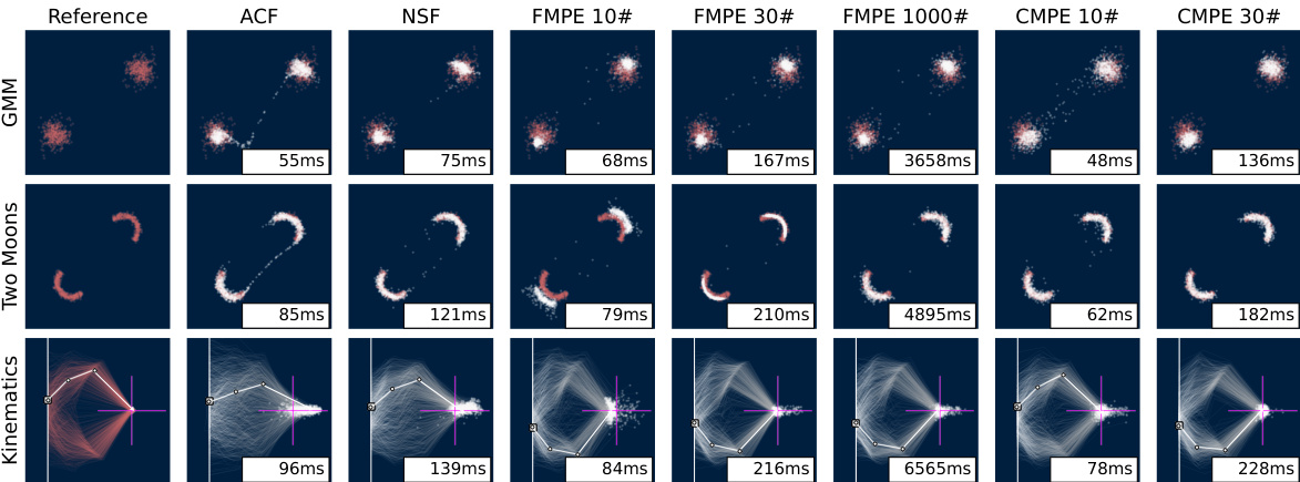
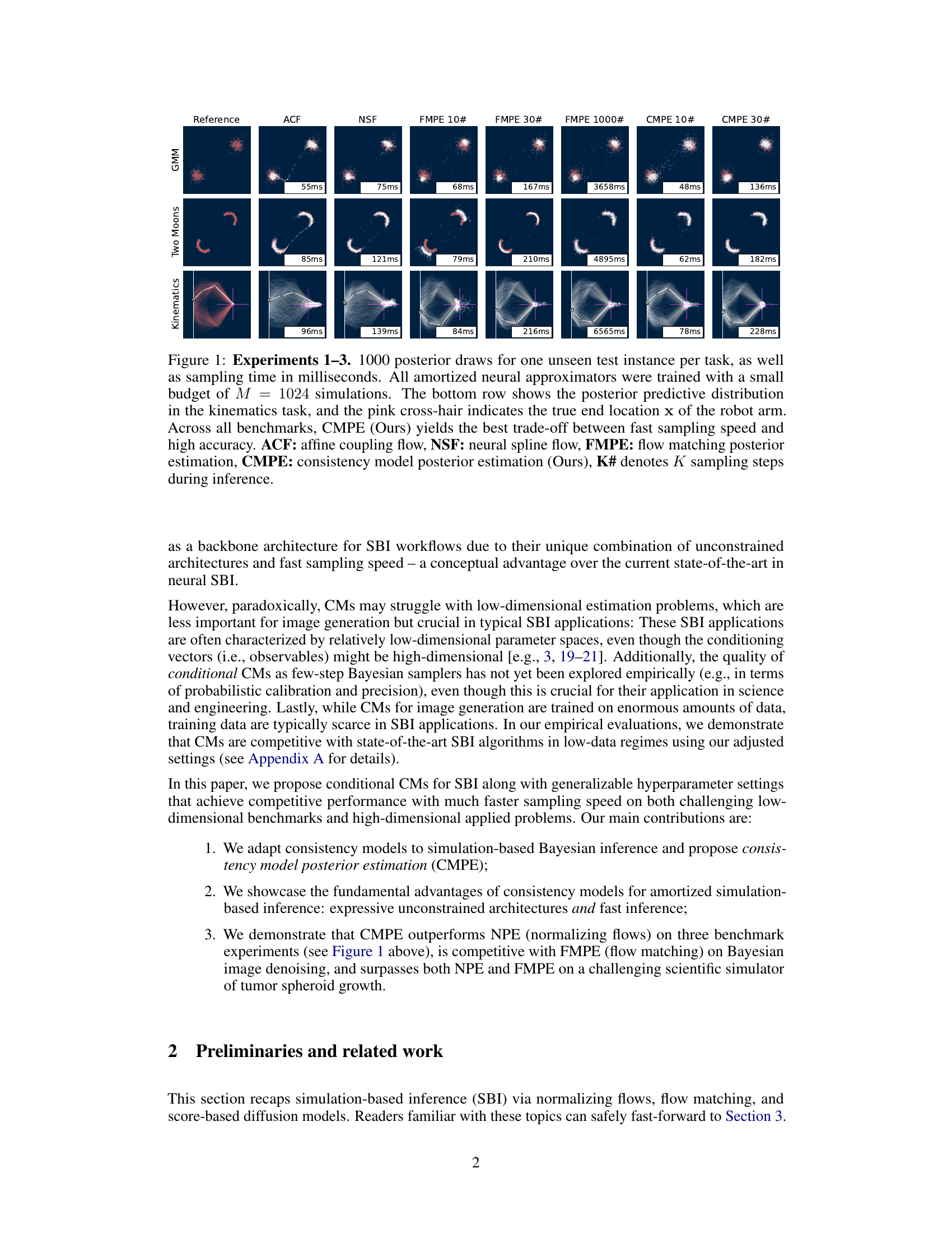
This figure presents a comparison of different posterior estimation methods (ACF, NSF, FMPE, CMPE) on three benchmark tasks: Gaussian Mixture Model (GMM), Two Moons, and Inverse Kinematics. For each method and task, 1000 posterior samples are drawn for a single unseen test instance. The sampling time (in milliseconds) is shown for each method. The bottom row visualizes the posterior predictive distribution for the inverse kinematics task, highlighting the true value with a pink crosshair. The results demonstrate that CMPE achieves the best balance between accuracy and sampling speed.

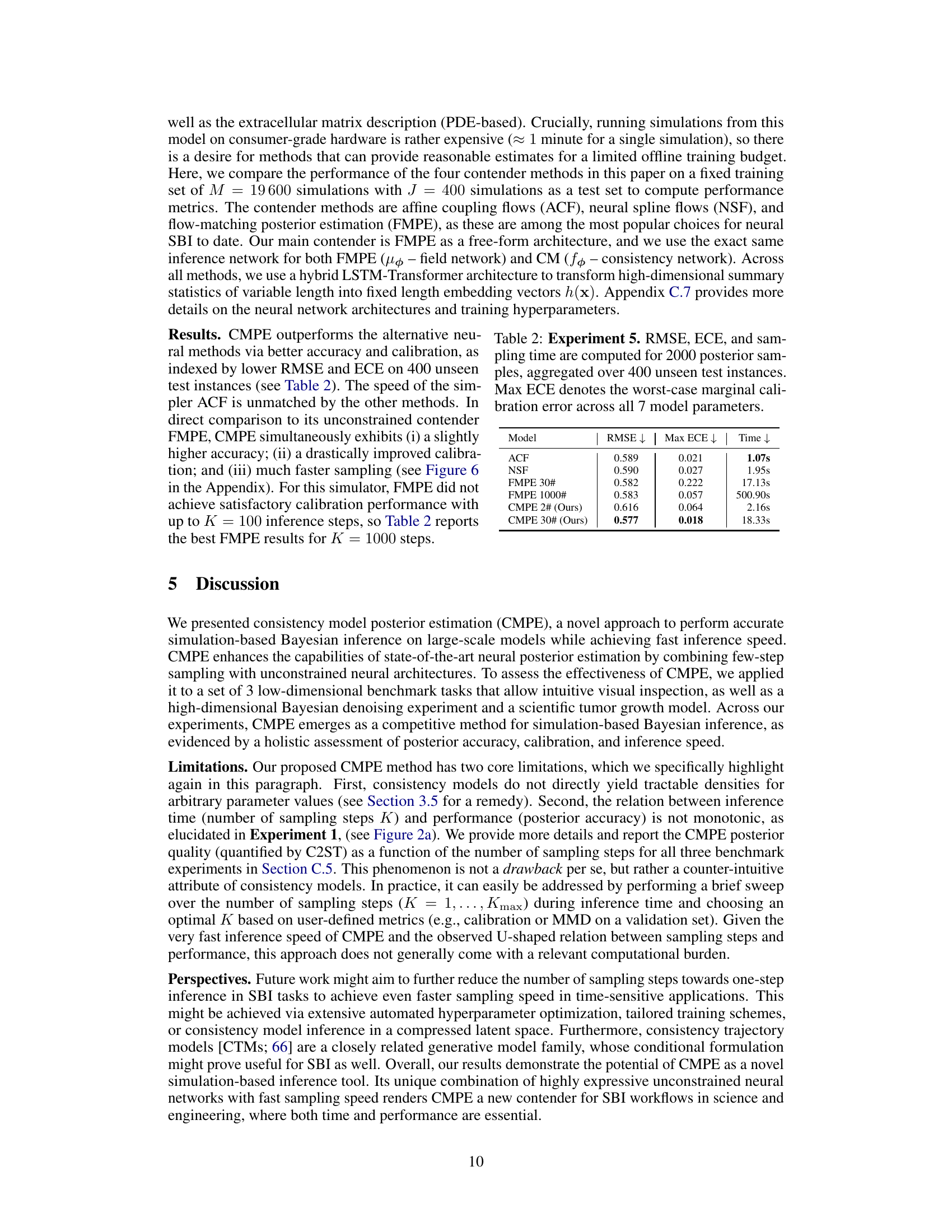
This table presents a quantitative comparison of the performance of CMPE and FMPE on the Fashion MNIST Bayesian denoising task. It shows the RMSE (Root Mean Squared Error), MMD (Maximum Mean Discrepancy), and time per sample for both models using two different neural network architectures (a naïve architecture and a U-Net architecture) and two different training set sizes (2000 and 60000 images). Lower RMSE and MMD values indicate better performance, and shorter time per sample indicates faster inference.
In-depth insights#
CMPE: SBI Sampler#
CMPE, presented as a novel SBI sampler, offers a compelling approach to posterior estimation by combining the strengths of unconstrained neural architectures with the efficiency of few-step sampling. Its design, inheriting advantages from consistency models, allows for flexible tailoring to various problem structures, overcoming the sampling inefficiency often associated with other unconstrained methods. CMPE’s capacity for rapid few-shot inference is a significant improvement, especially valuable for high-dimensional problems and scenarios with limited data. The paper demonstrates CMPE’s competitiveness with state-of-the-art algorithms on challenging low-dimensional benchmarks. Its superior speed is particularly noteworthy, offering a decisive advantage in real-world applications where computational efficiency is paramount. However, it’s important to note that CMPE’s performance relative to existing methods such as FMPE can vary based on the specific characteristics of the problem and dataset. While generally highly efficient, additional investigation into its performance in certain conditions is warranted.
CMPE Efficiency#
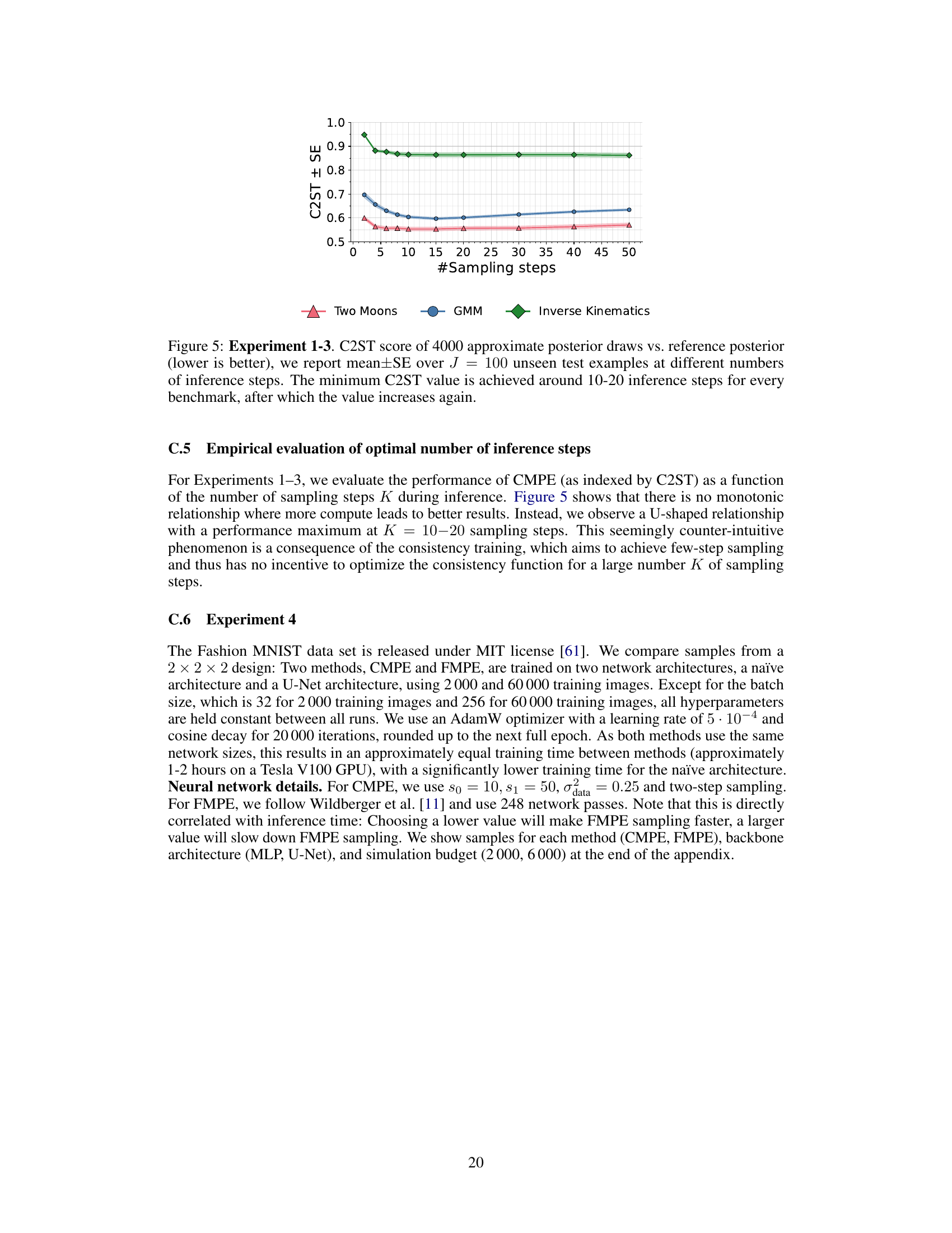
CMPE’s efficiency stems from its clever combination of unconstrained neural network architectures and a fast, few-step sampling process. Unconstrained architectures allow for greater flexibility in modeling complex posterior distributions, avoiding the limitations of invertible transformations found in methods like normalizing flows. The few-step sampling drastically reduces computational cost during inference compared to score-based diffusion models or flow matching, which require numerous iterative steps. This efficiency is particularly beneficial in high-dimensional or computationally expensive simulation settings common in scientific applications. The hyperparameter tuning strategies suggested contribute further to the model’s efficient and effective performance, particularly in data-scarce situations. However, the relationship between inference speed and sampling quality shows a non-monotonic U-shaped curve, suggesting an optimal number of sampling steps exists. Thus, while CMPE offers significant speed advantages, careful consideration of this trade-off is necessary for optimal results.
Low-D SBI#
Low-dimensional simulation-based inference (Low-D SBI) presents unique challenges and opportunities. The curse of dimensionality is less pronounced, allowing for potentially simpler models and faster computations compared to high-dimensional problems. However, these advantages must be carefully considered; while computationally efficient, Low-D SBI methods may struggle with complex posterior distributions or insufficient data. Careful selection of appropriate models and sampling techniques is crucial to avoid overfitting or poor estimation. The paper’s focus on improving the efficiency of SBI methods has significant implications for Low-D applications by potentially reducing computational costs and enabling more extensive analysis within limited computational resources. Further research should investigate the limitations of standard methods in the low-dimensional regime and develop tailored algorithms to exploit the specific characteristics of Low-D problems. Ultimately, balancing the advantages of simplicity with the need for accuracy is vital in Low-D SBI.
CMPE Limitations#
CMPE, while demonstrating promising results in simulation-based inference, exhibits limitations primarily concerning density estimation and the non-monotonic relationship between sampling steps and performance. The inability to directly evaluate the posterior density at arbitrary parameter values is a significant hurdle, restricting the model’s applicability for downstream tasks that rely on such evaluations. This necessitates reliance on surrogate density estimators or other workarounds. Furthermore, the non-monotonic relationship between the number of sampling steps and the quality of the posterior requires careful tuning and potentially compromises the speed advantage often touted for the model. While the authors suggest strategies to mitigate these limitations, such as exploring surrogate methods for density estimation and performing a sweep over various sampling steps during inference, these approaches add complexity and potential computational overhead, partially offsetting CMPE’s efficiency gains. Addressing these shortcomings is critical to further advance the model’s practical utility and broad adoption in SBI applications.
Future of CMPE#
The future of Consistency Model Posterior Estimation (CMPE) looks promising, particularly given its demonstrated speed and accuracy advantages in various applications. Further research should focus on addressing limitations such as the non-monotonic relationship between sampling steps and performance, and developing methods for direct density evaluation. Exploring the use of CMPE with other generative models, and adapting CMPE for specific applications with limited data, will significantly broaden its applicability. Investigating alternative training methods and hyperparameter optimization techniques could lead to even more robust and efficient models. Finally, exploring the potential of CMPE in high-dimensional settings and tackling complex scientific problems with scarce data would solidify its place as a leading method for simulation-based inference. Improving the theoretical understanding of CMPE, and proving bounds on its performance, would enhance the credibility and adoption of this method.
More visual insights#
More on figures

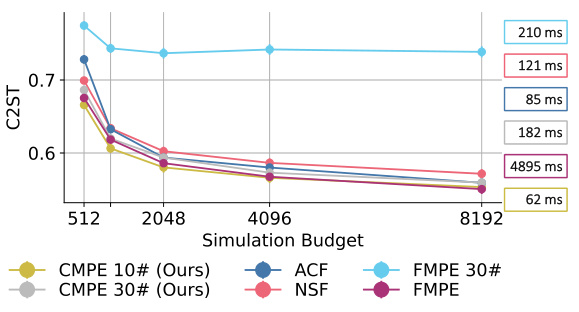
This figure compares the performance of CMPE against other methods (ACF, NSF, FMPE) on two benchmark tasks: Gaussian Mixture Model and Two Moons. The x-axis represents the sampling speed, and the y-axis shows the C2ST score, a measure of how well the approximated posterior matches the true posterior distribution (lower is better). Panel (a) shows CMPE outperforming other methods on the Gaussian Mixture Model, demonstrating both speed and accuracy improvements. Panel (b) shows CMPE with 10 sampling steps maintaining a performance edge on the Two Moons benchmark up to a training budget of 4096 simulations, indicating its efficiency in low-data settings.
This figure compares different methods for posterior estimation on three benchmark tasks: Gaussian Mixture Model, Two Moons, and Inverse Kinematics. The results show the posterior predictive distributions obtained by each method, along with their sampling times. CMPE is shown to be faster and more accurate than other methods.

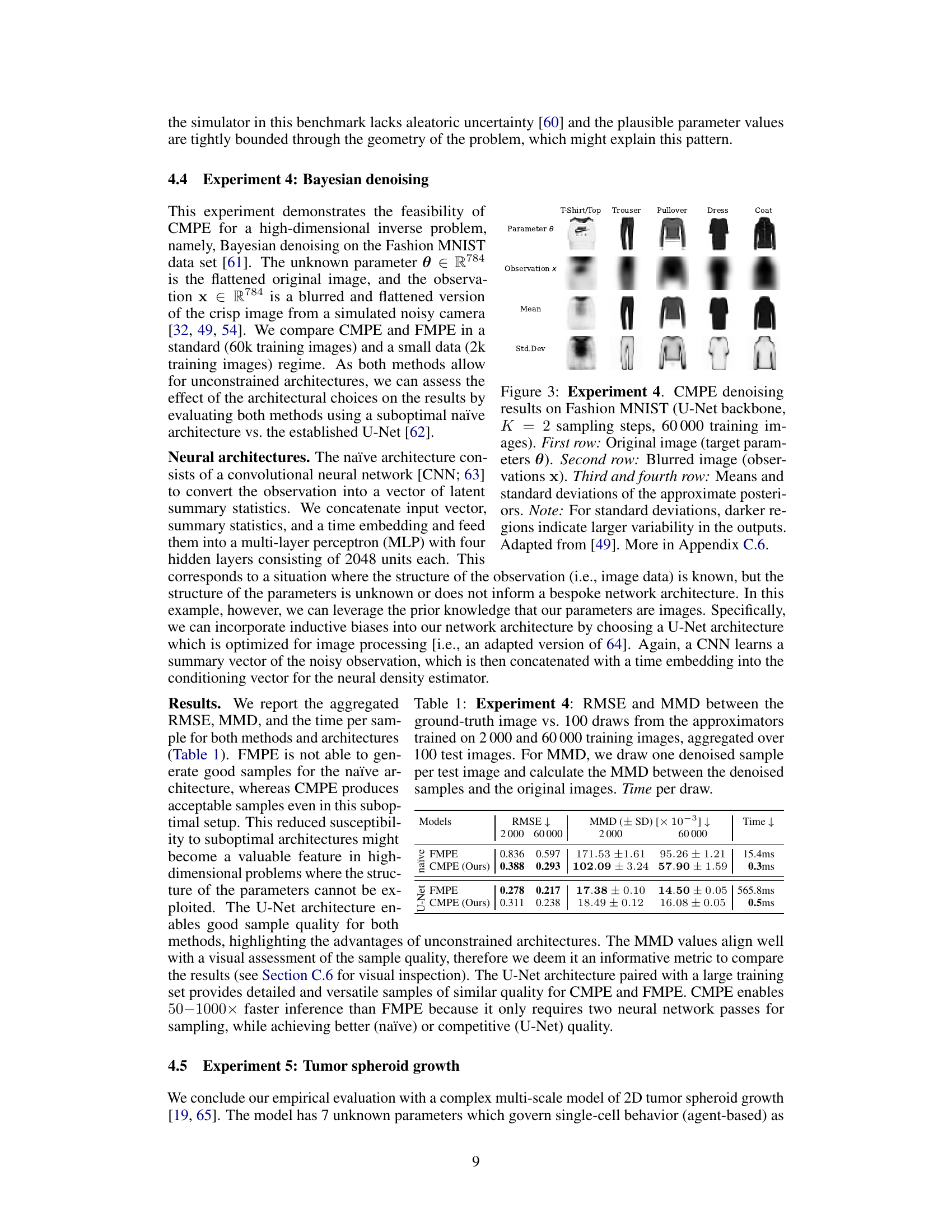
This figure shows the results of the Bayesian denoising experiment using CMPE on the Fashion MNIST dataset. It compares the original images (ground truth) to their blurred versions (observations) and then presents the mean and standard deviation of the posterior distribution estimated using CMPE. Darker shades in the standard deviation plots represent higher variability in the model’s predictions.

This figure compares the performance of different posterior estimation methods (ACF, NSF, FMPE, CMPE) on three benchmark tasks (Gaussian Mixture Model, Two Moons, and Inverse Kinematics). Each method’s posterior predictive distribution is visualized, along with the sampling time. CMPE consistently shows superior performance in terms of both accuracy and speed, especially for fewer sampling steps.

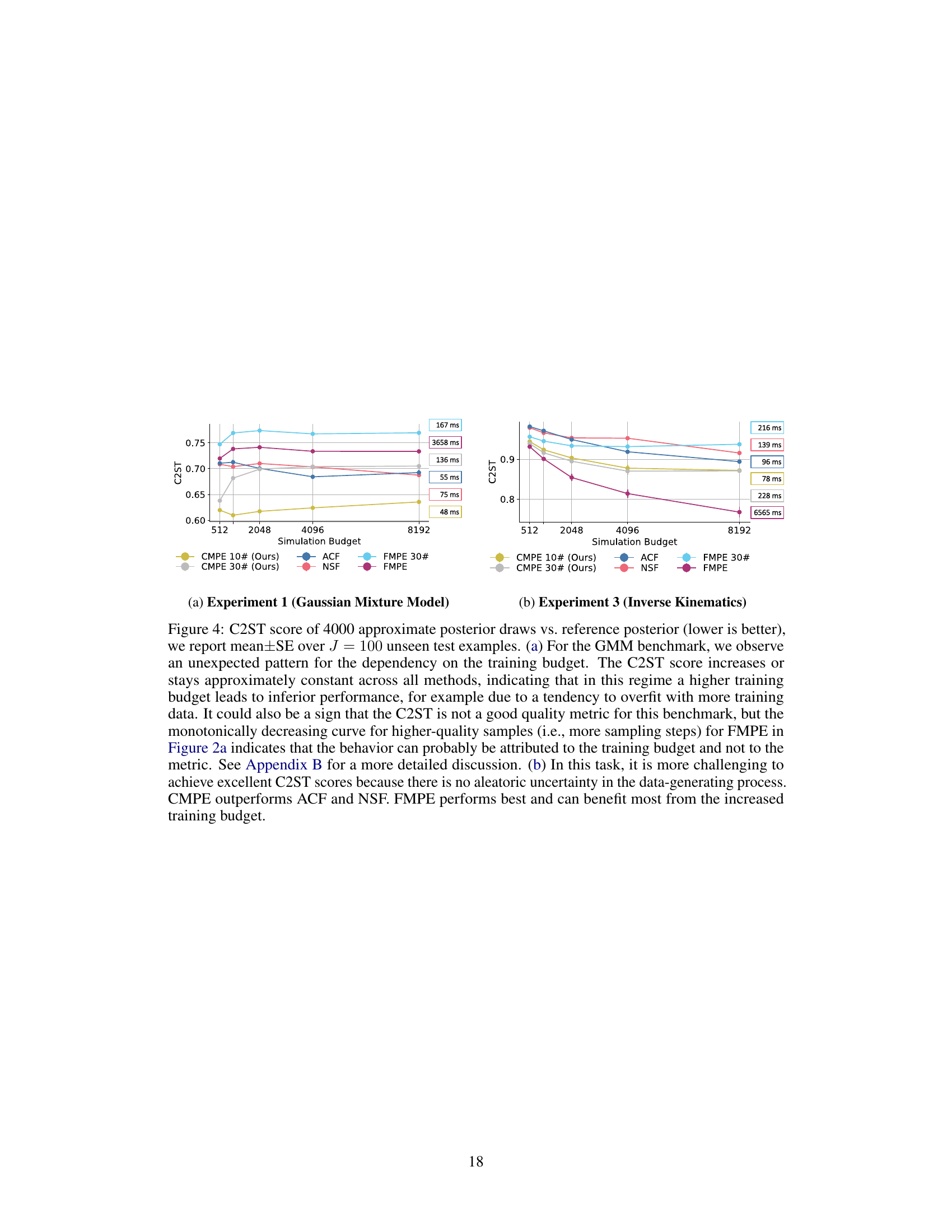
The figure shows the C2ST score (lower is better) for Gaussian Mixture Model and Two Moons benchmarks as a function of the simulation budget. CMPE consistently outperforms other methods in both speed and accuracy, especially for smaller training budgets.
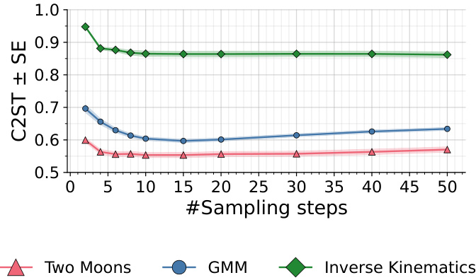
The figure shows the C2ST score for three different benchmarks (Two Moons, GMM, Inverse Kinematics) as a function of the number of sampling steps used during inference with CMPE. The C2ST score, measuring the accuracy of the posterior approximation, shows a U-shaped curve for all benchmarks. The optimal number of sampling steps is around 10-20 for all three experiments, indicating a sweet spot for balancing speed and accuracy.

This figure compares the performance of CMPE and FMPE on a complex tumor growth model. The plots show the posterior distributions for two parameters (log division depth and log division rate). CMPE shows accurate and unbiased estimations using only 30 sampling steps, which is significantly faster than FMPE, even when FMPE uses 1000 sampling steps. While the 1000-step FMPE eventually produces a better result, CMPE’s speed advantage is quite significant.

This figure shows the calibration plots for each of the methods used in Experiment 5 (Tumor Spheroid Growth). The plots show the ranked probability scores against the fractional rank statistics. The shaded area represents the 95% confidence interval for perfect calibration. The inference times (in seconds) required to draw 2000 posterior samples are also provided for each method. Green indicates the best performance, while dark red represents the worst for each metric.

This figure presents calibration plots for Experiment 5, evaluating the performance of four different methods (ACF, NSF, FMPE, CMPE) in estimating the posterior distribution of a complex tumor spheroid growth model. Each plot shows the rank-frequency distribution (ECDF) for each parameter, comparing the posterior samples generated by each method against the true posterior. The gray shaded area represents the 95% confidence interval for perfect calibration, and green/darkred indicate best/worst performance per metric. Inference times (in seconds) for generating 2000 posterior samples are also provided, highlighting CMPE’s speed advantage.

This figure displays calibration plots for each of the five methods compared in Experiment 5 of the paper. The gray shaded areas represent the 95% confidence intervals for proper calibration. The plots show the fractional rank statistic which is a measure of the accuracy of the calibration. The inference time, in seconds, for obtaining 2000 posterior samples is also given. The best performing method for each metric is highlighted in green, while the worst-performing is in dark red. The goal of the experiment is to evaluate the methods on a complex, computationally-expensive scientific simulator, comparing both accuracy, calibration and inference speed.

This figure presents calibration plots for Experiment 5, which involved a complex multi-scale model of 2D tumor spheroid growth. The plots show the results from different methods: Affine Coupling Flow (ACF), Neural Spline Flow (NSF), Flow Matching (FMPE) with 30 and 1000 steps, and Consistency Model Posterior Estimation (CMPE) with 2 and 30 steps. The gray shaded areas represent 95% confidence intervals for proper calibration. The inference times (wall-clock time in seconds) needed to generate 2000 posterior samples for each method are also shown. Green indicates the best performance, while dark red shows the worst performance. The figure highlights CMPE’s faster inference compared to other methods.

This figure displays calibration plots obtained from Experiment 5, evaluating the performance of four methods: Affine Coupling Flow, Neural Spline Flow, Flow Matching (with 30 and 1000 steps), and Consistency Model (with 2 and 30 steps). Each method’s calibration is visually assessed using rank ECDFs and 95% confidence bands, showing the discrepancy between the model’s predicted uncertainty and actual uncertainty. Inference times (in seconds) for drawing 2000 samples are also indicated. The figure helps to compare the calibration accuracy and efficiency of the different methods, highlighting CMPE’s superior performance.

This figure displays calibration plots for five different methods used in Experiment 5 of the paper, which focuses on a complex multi-scale model of 2D tumor spheroid growth. The plots show the calibration of uncertainty estimates for each method using rank histograms. The gray shaded regions indicate 95% confidence intervals for perfect calibration. The best performing method (lowest RMSE and ECE) for each metric is highlighted in green, while the worst is shown in dark red. Inference time for each method is also reported, illustrating the relative speed of each.
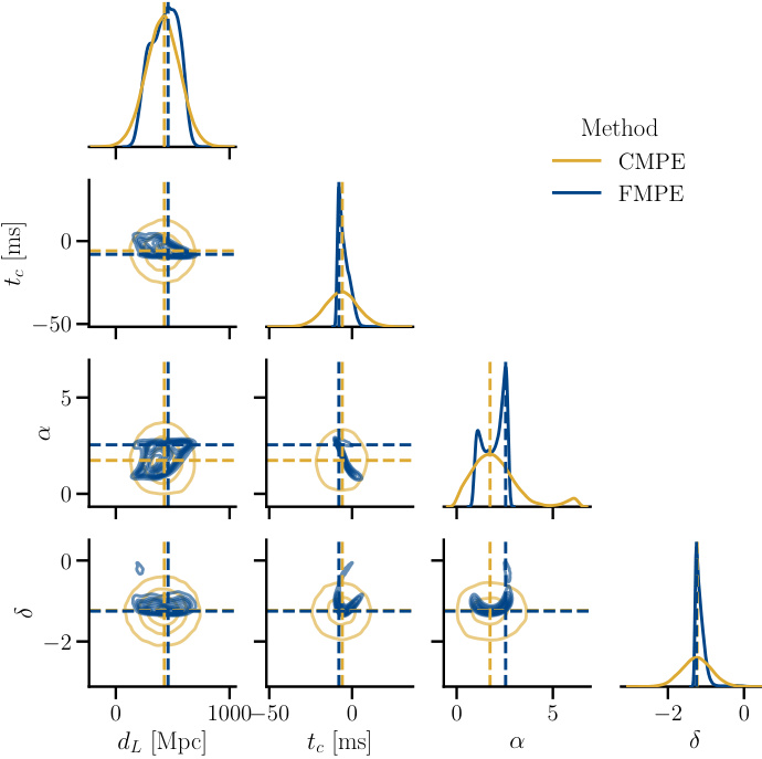
This figure shows a pairplot of the univariate and bivariate posterior distributions obtained using both CMPE and FMPE methods. The plot reveals that FMPE significantly outperforms CMPE in capturing the nuances of the posterior distribution. The CMPE posteriors appear underexpressive and lack the detail present in the FMPE posteriors. This suggests a limitation of CMPE in certain applications where fine-grained details are crucial.

This figure shows the results of applying the CMPE model with a U-Net architecture to the Fashion MNIST dataset. The model was trained on only 2000 images. Each row shows a different class from the Fashion MNIST dataset. The leftmost column displays the ground truth image (Param. θ), followed by the noisy observation (Obs. x), and then five different samples generated by the model (Sample). This illustrates the model’s ability to denoise images, even with a limited training set.

This figure displays the results of applying the CMPE model with a U-Net architecture to the Fashion MNIST dataset for image denoising. It shows the original images (Param. θ), the noisy input images (Obs. x), and five samples generated by CMPE for each class, illustrating the model’s ability to reconstruct the original image from a noisy version. The experiment used a limited training dataset of 2000 images.

This figure shows the results of applying the CMPE method with a U-Net architecture to the Fashion MNIST dataset for image denoising. The experiment used a small training set of 2000 images and a two-step sampling process. Each row represents a different class from the Fashion MNIST dataset, showing the original image (Param. θ), the noisy observation (Obs. x), and several samples generated by CMPE. The samples demonstrate the model’s ability to reconstruct the original image from the noisy input.

This figure shows the results of applying the CMPE method with a U-Net architecture and two-step sampling on the Fashion MNIST dataset. The dataset consists of images from 10 different clothing categories, each with a blurred version representing noisy observations. The figure displays, for each category, the original image (Param. θ), the noisy observation (Obs. x), and five denoised samples generated by CMPE. The experiment used a small training set of only 2000 images.
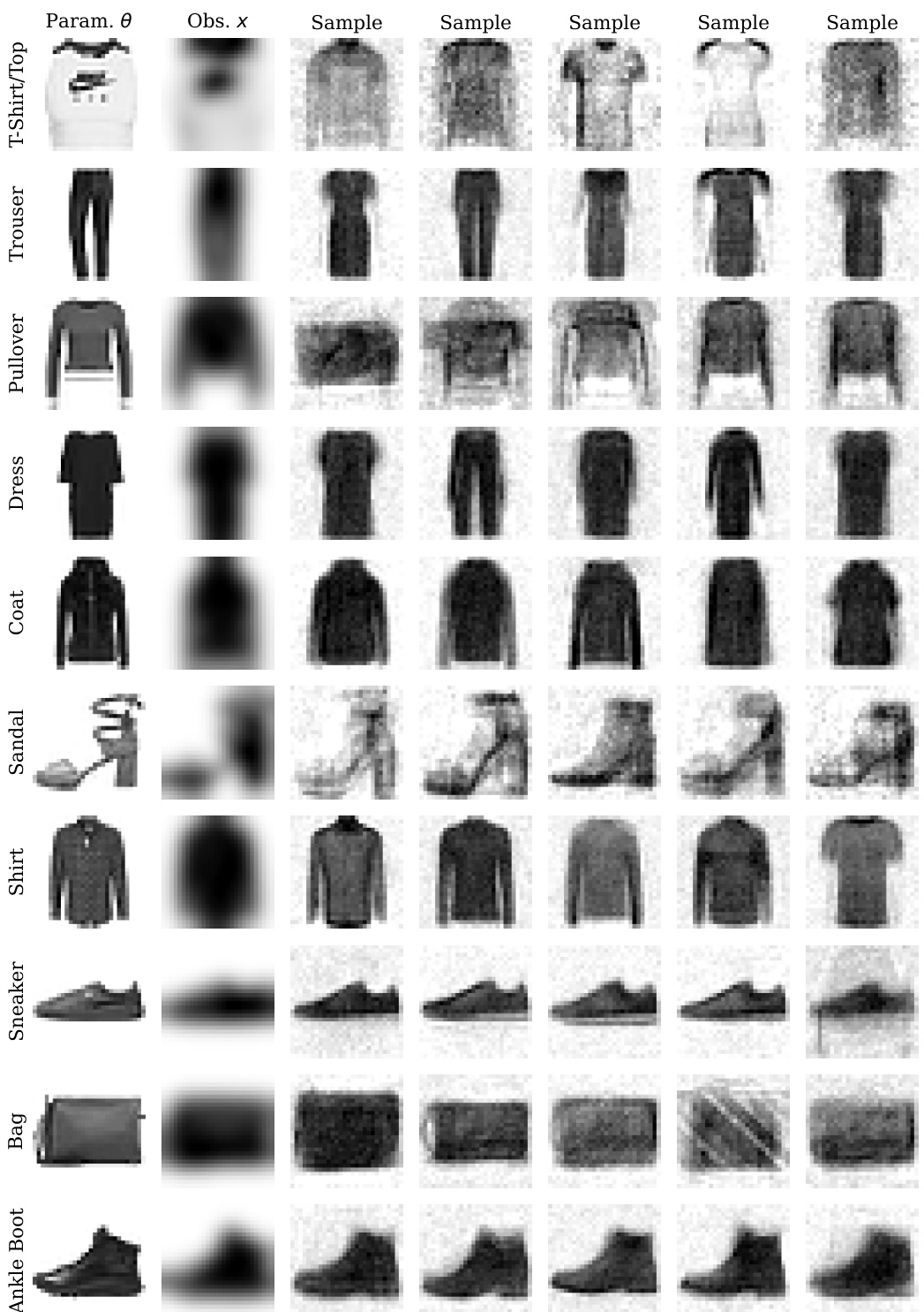
This figure shows the results of applying the CMPE method with a U-Net architecture to the Fashion MNIST dataset for image denoising. A small training set of 2000 images was used. For each class of clothing in the dataset, the figure displays the true image (Param. θ), the blurred noisy image (Obs. x), and 5 denoised samples generated by the model (Sample). This allows visualization of the model’s ability to reconstruct the original image from noisy data.

This figure shows the results of applying the CMPE method with a U-Net architecture to the Fashion MNIST dataset for image denoising. A small training set of 2000 images was used. The figure displays the true parameter (original image), the noisy observation (blurred image), and multiple samples from the posterior distribution generated by CMPE for each class of clothing in the dataset. This demonstrates the model’s ability to reconstruct the original images from the noisy input.
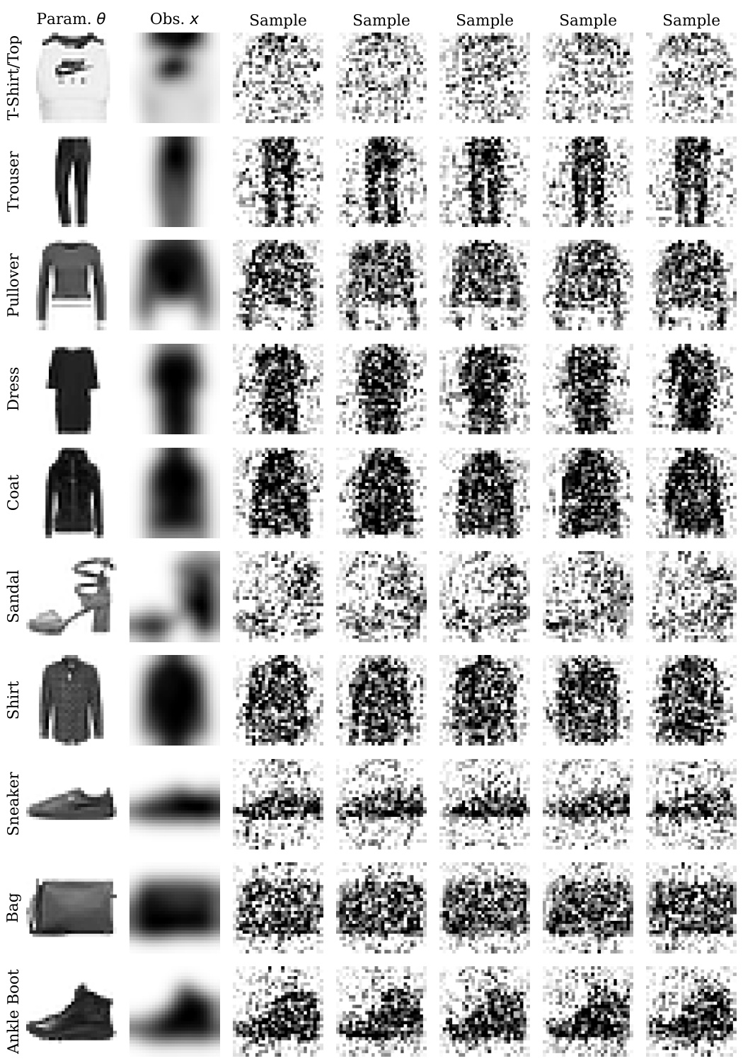
This figure shows the results of using the CMPE method with a U-Net architecture on the Fashion MNIST dataset. The experiment used a small training set of 2000 images and employed a two-step sampling process during inference. Each row presents a different class from Fashion MNIST, displaying the original parameter (θ), the noisy observation (x), and several posterior samples generated by CMPE. This illustrates the model’s ability to reconstruct images from noisy input.
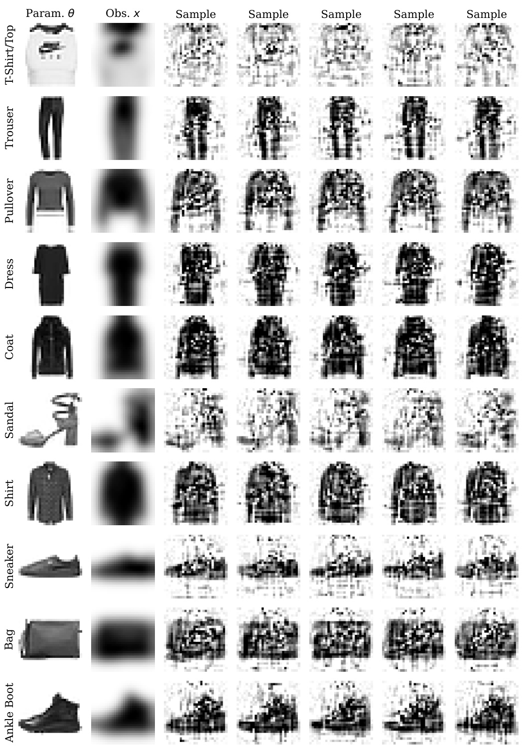
This figure shows the results of applying the CMPE method with a U-Net architecture to the Fashion MNIST dataset for image denoising. The experiment used a small training set of 2000 images and employed two-step sampling. For each class in the dataset, the figure displays the original image (Param. θ), the blurry observed image (Obs. x), and five samples generated by CMPE to illustrate the quality of the denoised images.
More on tables

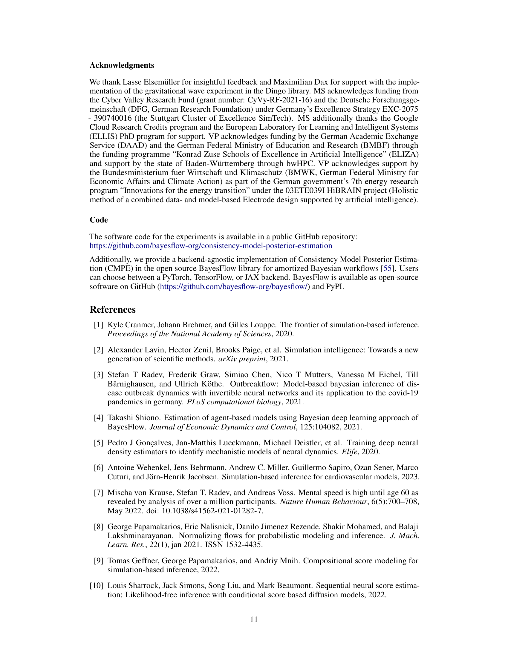
This table presents the results of Experiment 5, comparing different methods on a complex multi-scale model of 2D tumor spheroid growth. It shows the Root Mean Squared Error (RMSE), Expected Calibration Error (ECE), and sampling time for each method. Lower RMSE and ECE values indicate better accuracy and calibration, respectively, while lower time indicates faster inference. The ‘Max ECE’ column shows the worst marginal calibration error across all 7 parameters of the model.

This table details all functions and parameters required for training the consistency model. It specifies the loss metric, discretization scheme, noise schedule, weighting function, skip connections, and various parameters used in the training process. The values are largely adopted from Song and Dhariwal [46], with some modifications noted in the paper’s text.
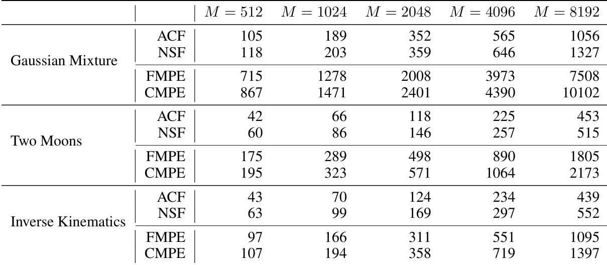
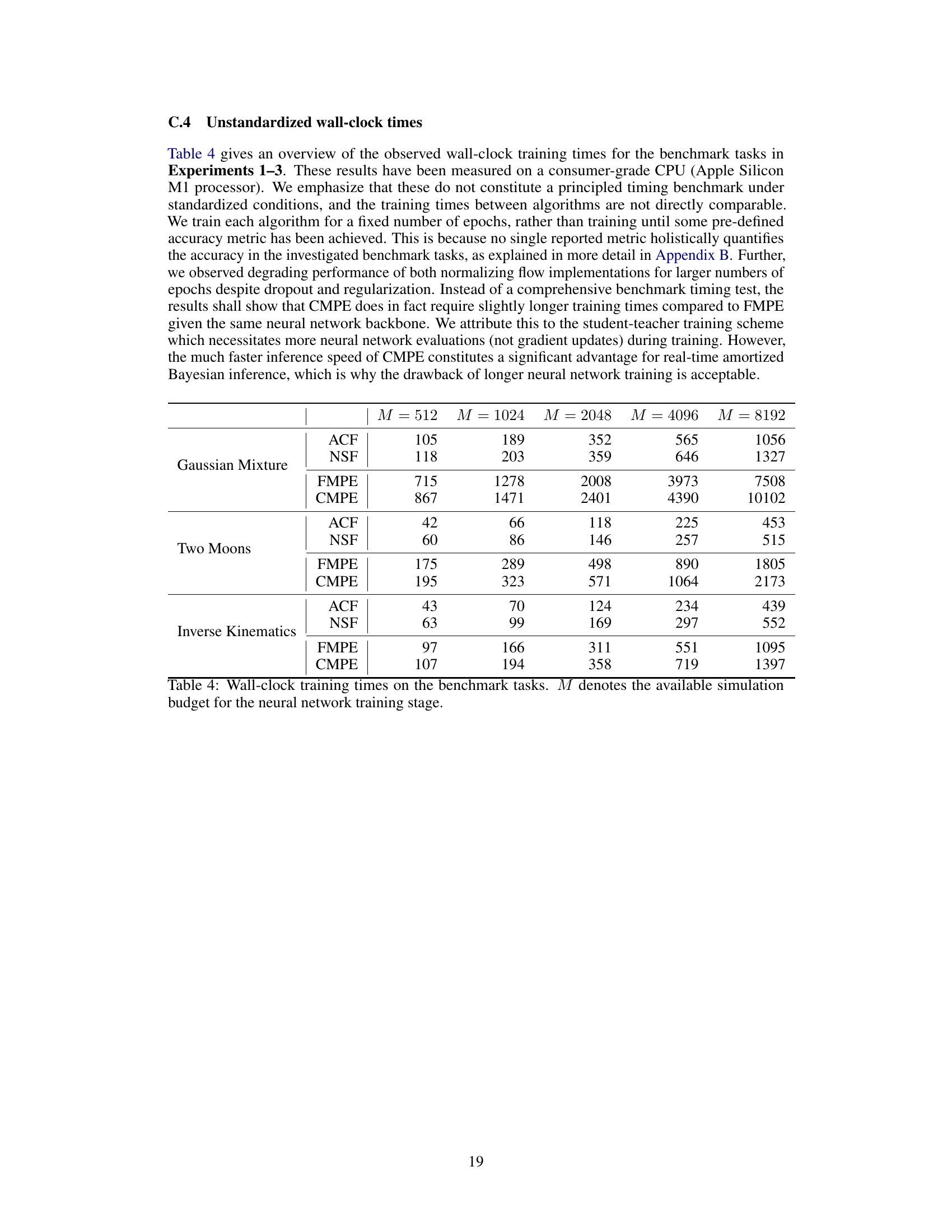
This table shows the training times for four different methods (ACF, NSF, FMPE, CMPE) across three benchmark tasks (Gaussian Mixture, Two Moons, Inverse Kinematics) and various simulation budget sizes (M). The training times are measured on a consumer-grade CPU and are not directly comparable across algorithms due to differences in training procedures and stopping criteria. The table highlights that while CMPE requires slightly longer training time than FMPE, its significantly faster inference speed makes it more suitable for real-time applications.
Full paper#
