↗ OpenReview ↗ NeurIPS Homepage ↗ Chat
TL;DR#
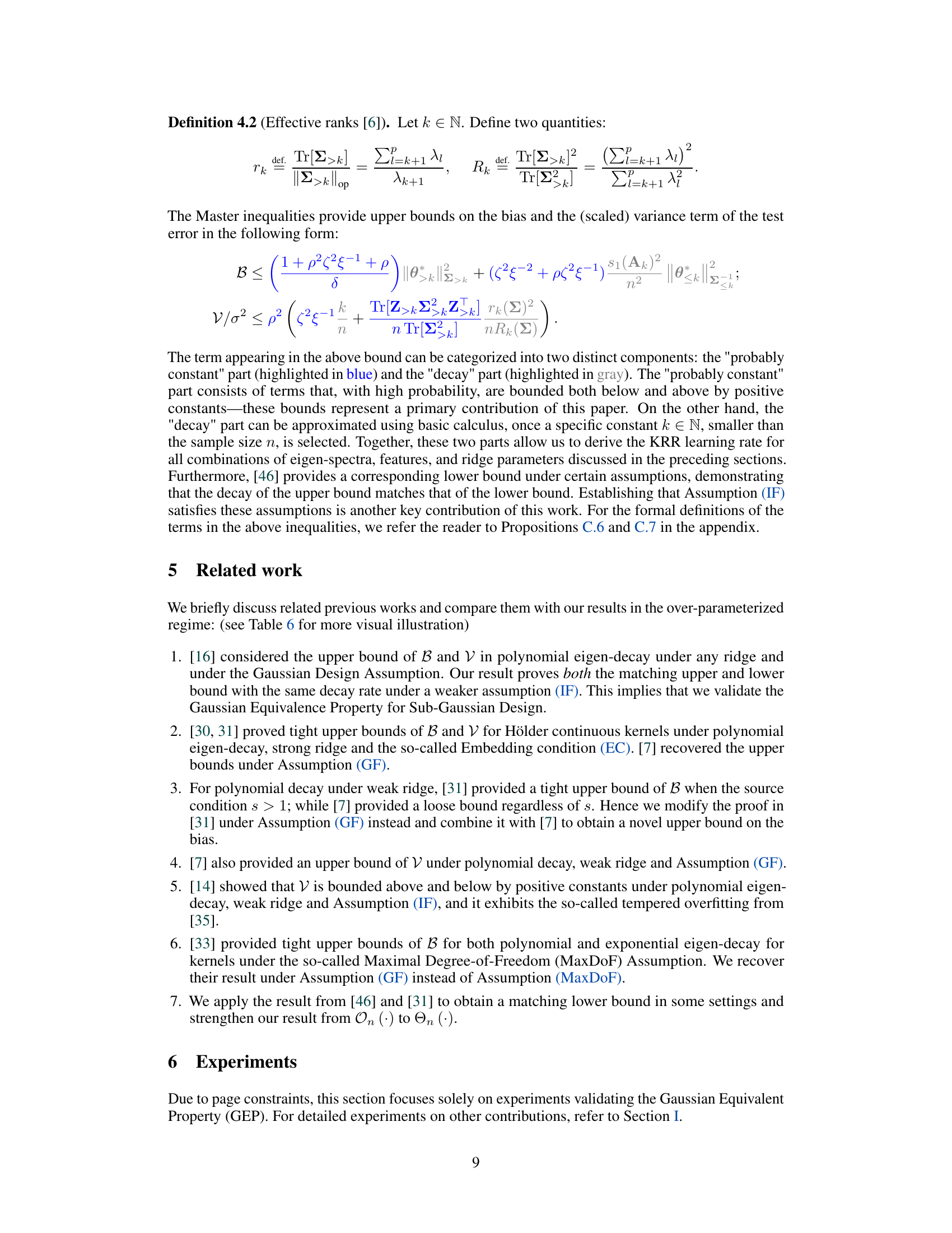
Kernel ridge regression (KRR) is a fundamental machine learning technique, but its learning curve’s behavior under various conditions remains incompletely understood. Previous studies often relied on the Gaussian Design Assumption, which may not hold for real-world data. This paper aims to bridge this gap by analyzing KRR under minimal assumptions. The core issue is that previous analyses often oversimplified the problem by making strong assumptions about the nature of the data and the kernel function. This limits their applicability and doesn’t fully capture the nuances of real-world scenarios.
This research presents a unified theoretical framework for understanding KRR’s test error, addressing various scenarios involving independent or dependent feature vectors, different kernel properties (eigen-decay rates and eigenfunction characteristics), and varying levels of regularization. The study validates the Gaussian Equivalence Property and provides novel, improved generalization error bounds across a broad range of settings. These contributions advance our understanding of KRR’s generalization behavior and potentially inform the development of more efficient and effective machine learning algorithms.
Key Takeaways#
Why does it matter?#
This paper is crucial for researchers in machine learning and statistics. It unifies existing theories on kernel ridge regression, improves generalization error bounds, and validates the Gaussian Equivalence Property, which is foundational for understanding deep learning. It opens avenues for research into minimal-assumption generalization analysis and deep network theory.
Visual Insights#
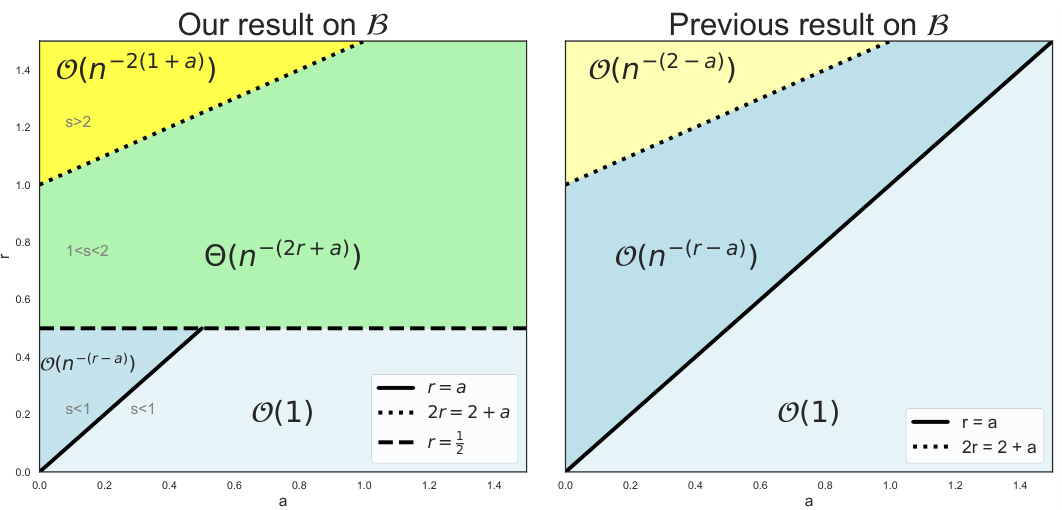
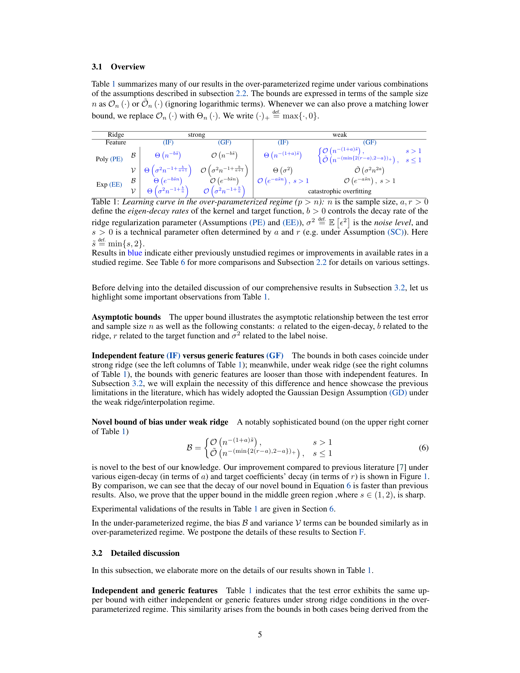
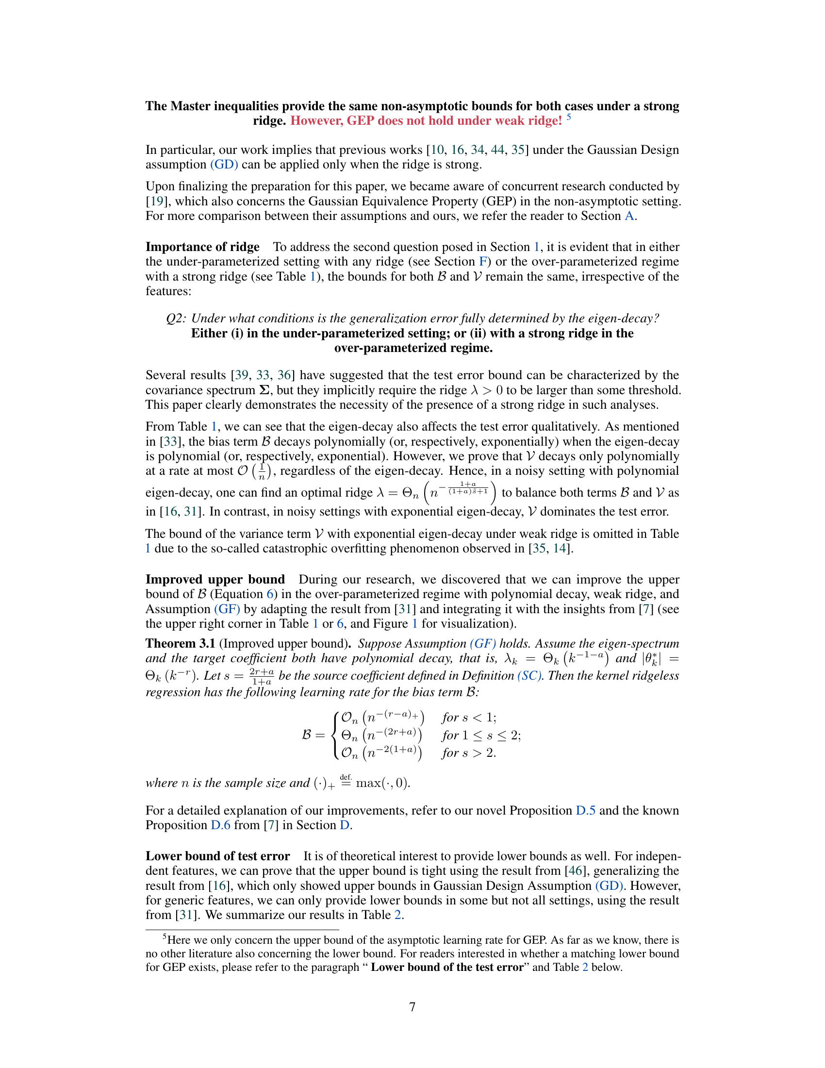
This figure shows a comparison of bias term upper bounds under weak ridge and polynomial eigen-decay conditions. The left plot represents the improved upper bound from the current paper (Propositions D.5, D.6, and E.1), while the right plot displays the previous result from reference [7] (Proposition D.6). The plots are phase diagrams showing how the upper bound changes with respect to the source coefficient (s) and a parameter (a) related to eigen-decay rate. The gray shaded regions in the left plot indicate the range of the source coefficient in different settings.

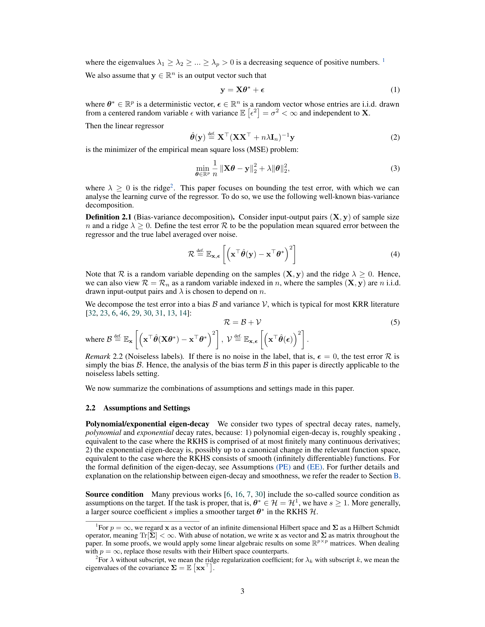
This table summarizes the results of the over-parameterized regime (p>n) of kernel ridge regression. It shows the asymptotic upper bounds for the bias and variance terms in the test error, expressed as functions of the sample size (n). The table considers various settings defined by combinations of polynomial/exponential eigen-decay, strong/weak ridge regularization, independent/generic features, and source coefficient (s). Improvements and novel results are highlighted in blue.
In-depth insights#
Kernel Eigen-decay#
The concept of kernel eigen-decay is crucial for understanding the generalization properties of kernel ridge regression (KRR). It essentially describes how quickly the eigenvalues of the kernel matrix decay. A faster decay often implies better generalization, as it suggests that the kernel is less prone to overfitting. This is because a fast decay indicates that the kernel’s eigenfunctions are concentrated on lower frequencies, effectively reducing the model’s complexity and its sensitivity to noise or irrelevant features. Conversely, a slow eigen-decay implies that the kernel can capture fine-grained details in the data, potentially resulting in overfitting. The relationship between eigen-decay and smoothness is also significant. Smoother kernels tend to have faster eigen-decay. Analyzing eigen-decay rates (polynomial, exponential) helps in determining the learning curve of KRR under various assumptions about the data and model parameters.
Gaussian Equivalence#
The concept of “Gaussian Equivalence” in kernel ridge regression (KRR) is a fascinating one, suggesting that the generalization performance of KRR is surprisingly similar whether the features are drawn from a true data distribution or from a simpler Gaussian distribution. This equivalence is particularly intriguing because real-world data rarely follows a Gaussian distribution. The paper investigates the conditions under which this equivalence holds, showing that strong ridge regularization is a crucial factor. This finding sheds light on the success of previous analyses that relied on the Gaussian design assumption, demonstrating that their results hold more broadly than previously thought. Furthermore, minimal assumptions are used in the analysis. The paper’s findings challenge previous oversimplifications and reveal a deeper understanding of KRR’s generalization behavior by providing novel theoretical bounds. The unification of different KRR learning curve scenarios is a valuable contribution, as well as demonstrating the validity and limitations of Gaussian Equivalence. This insight is both valuable for theoretical understanding and practical applications of KRR.
Unified Test Error#
A unified test error analysis in machine learning seeks to develop a single theoretical framework capable of explaining the generalization performance of a wide array of models and settings. This contrasts with the existing approaches that often rely on specific assumptions about the data generating process or model architecture. A unified theory would ideally provide bounds on the test error that hold across various regimes, including the overparameterized and underparameterized settings, and different types of data (e.g., independent and dependent features). Achieving such unification is crucial for a deeper understanding of generalization and could lead to improved algorithms and model selection techniques. Key challenges in developing such a unified theory include the complex interplay between model capacity, data distribution, and regularization, and the inherent difficulty in characterizing the generalization performance of complex models.
Strong vs. Weak Ridge#
The concept of “Strong vs. Weak Ridge” in kernel ridge regression hinges on the relationship between the regularization parameter (lambda) and the eigenvalues of the kernel matrix. A strong ridge implies lambda is significantly larger than the smallest eigenvalue, effectively dominating the kernel’s influence and leading to a simpler model with reduced variance and potentially increased bias. Conversely, a weak ridge signifies lambda is comparable to or smaller than the smallest eigenvalue, allowing the kernel to exert more influence, which might capture intricate data patterns more effectively (lower bias), but at the cost of increased variance and the potential for overfitting. The choice between strong and weak ridges is crucial in the bias-variance trade-off and impacts generalization performance. Strong ridges are often preferred in high-dimensional or noisy settings to prevent overfitting. However, weak ridges can be advantageous when dealing with small datasets or when the goal is to capture complex relationships, provided appropriate safeguards are in place to mitigate overfitting. The optimal choice depends heavily on the specific application, dataset properties, and the desired balance between bias and variance.
Future Research#
The paper’s “Future Research” section would ideally delve into several crucial areas. First, sharpening the theoretical upper bounds, particularly in the weak ridge regime, is vital. The current bounds appear somewhat loose, and tighter, more precise bounds would significantly strengthen the theoretical contributions. Second, extending the analysis to more complex kernel types beyond those considered in the paper is important. The paper focuses primarily on polynomial and exponential eigen-decay, but exploring other decay rates and kernel structures could broaden the applicability of the findings. Third, investigating the impact of different data distributions is critical. While the paper touches upon this, a more in-depth investigation into the influence of data structure on learning curves is necessary. Finally, rigorous empirical validation across various datasets and tasks is needed. The paper includes limited experimental validation, focusing mostly on GEP, and comprehensive empirical evaluation with diverse real-world data would significantly enhance the results’ generalizability and impact.
More visual insights#
More on figures

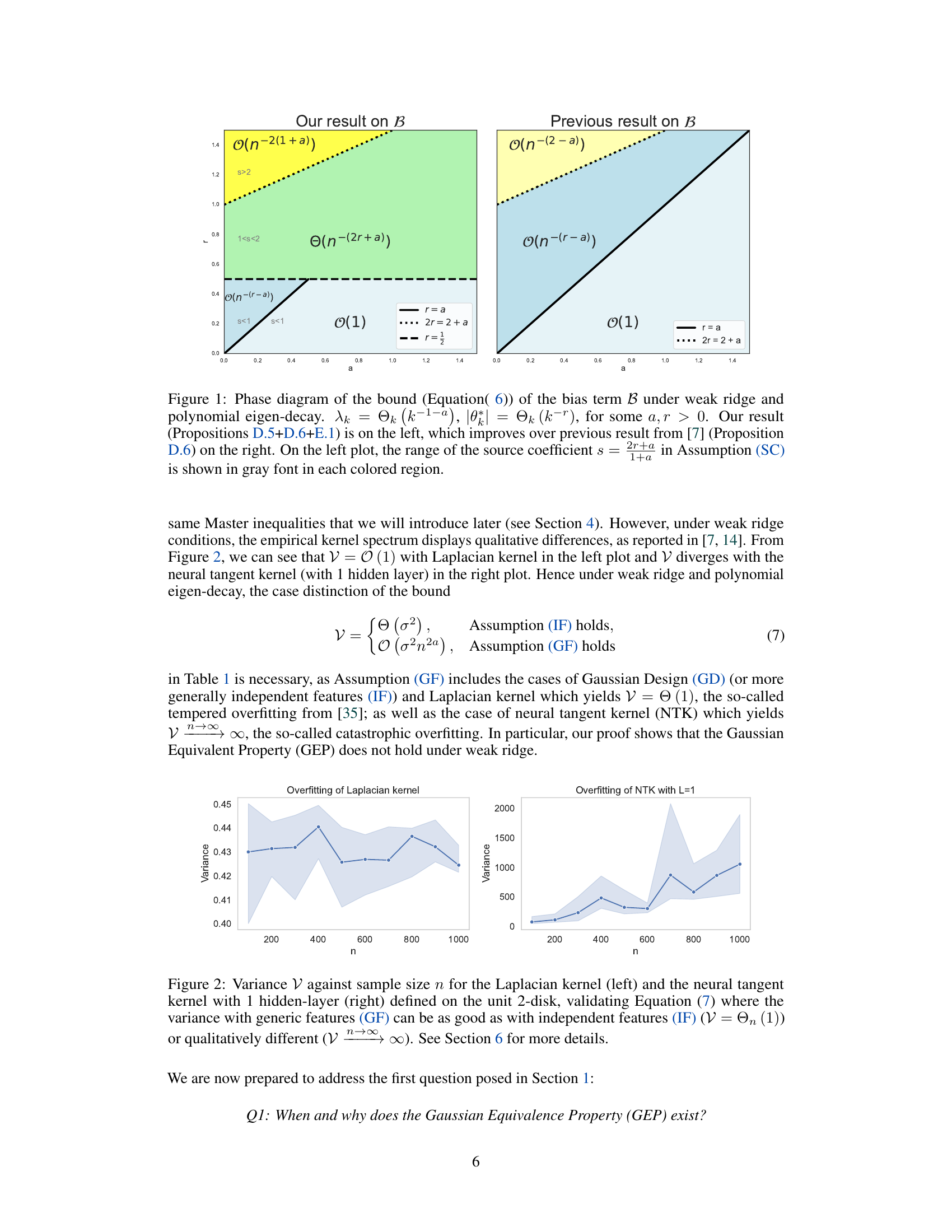
This figure displays the variance against sample size n for kernel ridge regression with no ridge regularization (λ = 0). Two different kernels are used: a Laplacian kernel and a Neural Tangent Kernel (NTK). The plot on the left shows that the Laplacian kernel exhibits tempered overfitting, meaning the variance remains relatively constant as the sample size increases. In contrast, the plot on the right shows catastrophic overfitting with the NTK, where the variance increases significantly with increasing sample size.
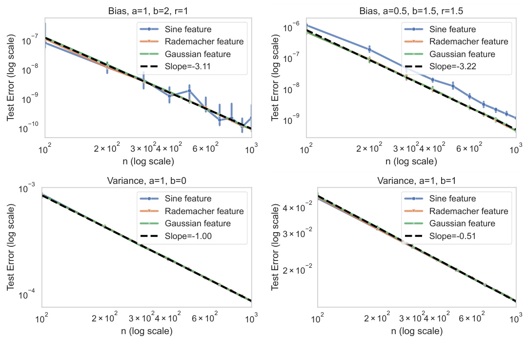
This figure shows the decay of bias and variance terms in the over-parameterized regime under different ridge decays and target coefficient decays. Three different feature types are used: sine features, Rademacher features and Gaussian features. The results demonstrate that all three features exhibit the same theoretical decay rate, thereby confirming the Gaussian Equivalence Property (GEP) in the context of independent features.
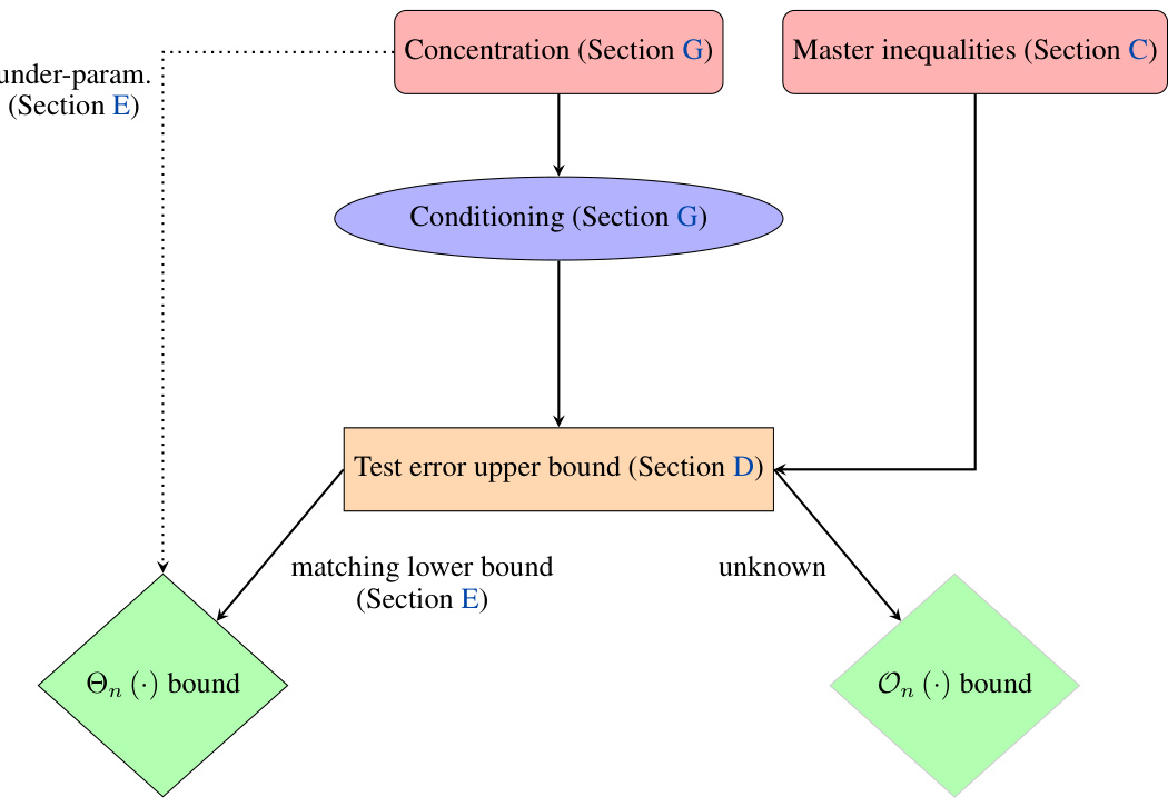
This flowchart summarizes the main steps and techniques used in the proofs presented in the paper. It shows how the concentration of features and conditioning, along with the master inequalities, are used to derive upper bounds for the test error in both the over- and under-parameterized regimes. The flowchart also highlights where matching lower bounds are proven and where they are still unknown.

This figure shows experimental results on the decay of bias and variance terms under various conditions. The experiment uses three different feature types: Sine features (representing dependent features), Rademacher features, and Gaussian features (both representing independent features). The results show that the bias and variance decay rates match theoretical predictions across all three feature types, supporting the Gaussian Equivalence Property (GEP) for independent features. Different panels show the results for different settings of the parameters in the eigen-decay rates and the ridge parameter.

This figure shows a comparison of the bias term bound (Equation 6) from this paper and a previous result from reference [7], under weak ridge regression and polynomial eigen-decay. The phase diagram illustrates the impact of source coefficient (s) and parameter (a) on the bias term bound. The left plot shows the improved bound from this paper, highlighting different regions based on source coefficient values. The right plot shows the previous result from [7]. Gray shaded regions in the left plot represent the range of the source coefficient ’s'.

This figure displays the decay of the bias term (B) under a strong ridge regularizer. Two settings are shown, differing in the values of a and r which affect the eigen-decay rate of the kernel and the decay rate of the target function respectively. In both settings, three types of feature vectors are used: Sine feature, Rademacher feature, and Gaussian feature. The results show that the bias term decays at the theoretically predicted rate for all three feature types, which supports the Gaussian Equivalence Property (GEP). The GEP states that the generalization performance remains the same whether using whitened kernel features or standard Gaussian vectors.

This figure shows the decay of the bias term B under weak ridge conditions for two different sets of parameters. The left panel shows a case where the source coefficient s is greater than 1, and the decay of the bias aligns with the theoretical prediction. The right panel shows a case where s is less than 1; here, the empirical decay of the bias is faster than the theoretical prediction, suggesting the theoretical bound might be too pessimistic in this regime.

This figure shows the decay of the variance term (V) under strong ridge conditions. Two plots are shown, each illustrating a different scenario resulting in different decay rates. The plots demonstrate the Gaussian Equivalent Property (GEP). The term V represents the variance of the test error, and its decay rate is influenced by the kernel’s eigen-decay, the target function’s properties, the ridge regularization strength, and the noise level. The theoretical decay rates are compared to experimental results using three types of features: Sine features, Rademacher features, and Gaussian features, showcasing the equivalence of generalization performance between the dependent (kernel) and independent features under strong ridge conditions.

This figure shows the variance against the sample size n for two different kernels under no ridge regularization. The left panel shows a Laplacian kernel, which exhibits tempered overfitting. The variance increases initially but then plateaus. The right panel shows the neural tangent kernel (NTK), which shows catastrophic overfitting. The variance continues to increase drastically with the sample size n.
More on tables

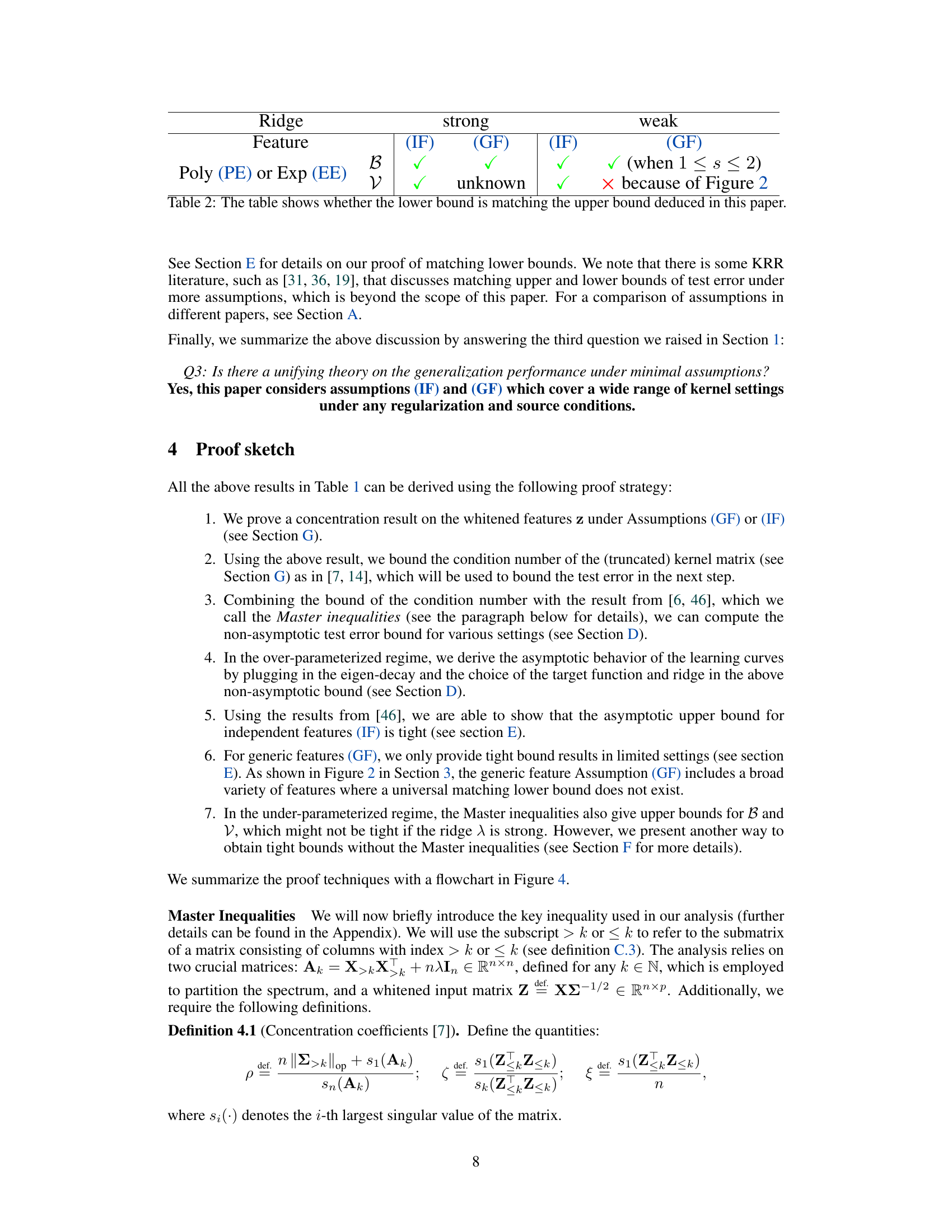
This table summarizes whether the lower bounds derived in the paper match the upper bounds for bias (B) and variance (V) in different settings of kernel ridge regression. The settings include strong vs. weak ridge regularization and independent vs. generic features. The table shows whether a matching lower bound could be proven for each setting, indicating the tightness of the upper bounds established in the paper.

This table summarizes the main results of the paper regarding the learning curve in the over-parameterized regime (when the number of features p is greater than the sample size n). It shows how the bias (B) and variance (V) terms of the test error decompose, depending on various factors: the type of eigen-decay (polynomial or exponential), the strength of the ridge regularization, whether the features are independent or generic, and the source condition (SC). The table also highlights novel bounds and improvements over existing results.

This table summarizes the main results of the paper regarding the learning curve of kernel ridge regression in the over-parameterized regime (p>n). It shows the asymptotic bounds (in terms of the sample size n) for the bias (B) and variance (V) terms of the test error under various combinations of assumptions regarding the kernel eigen-decay, ridge regularization, noise level, target function smoothness, and feature vector properties (independent or generic features). The table highlights improvements over existing bounds and identifies scenarios where the Gaussian Equivalence Property holds. The table also distinguishes between the strong and weak ridge regimes.
This table summarizes the main results of the paper regarding the learning curve in the over-parameterized regime (where the number of features p is greater than the sample size n). It shows how the bias (B) and variance (V) terms of the test error decompose, depending on various factors such as the type of eigen-decay (polynomial or exponential), the type of ridge regularization (strong or weak), whether the features are independent or generic, and the source condition (SC). The table provides asymptotic upper bounds (and in some cases matching lower bounds) on the test error expressed as a function of the sample size n and other relevant parameters. Results that improve upon or extend previous results are highlighted in blue.

This table summarizes the results of the analysis of the learning curve in the over-parameterized regime (p>n) under various combinations of assumptions and settings. It shows the asymptotic bounds of the bias (B) and variance (V) terms of the test error for both polynomial and exponential eigen-decay rates. The table also highlights the difference in bounds between independent and generic features, and how the results differ under strong and weak ridge regularization. Results in blue represent either previously unstudied cases or improvements over existing bounds.
Full paper#
