↗ OpenReview ↗ NeurIPS Homepage ↗ Chat
TL;DR#
Time series forecasting is critical across various domains. While Transformers have significantly advanced this field, their effectiveness is debated, with simpler linear models sometimes outperforming complex Transformer-based approaches. This highlights a need for more streamlined architectures and a deeper understanding of the role of different Transformer components. This paper addresses this by focusing specifically on self-attention’s effectiveness.
The researchers introduce a novel architecture called CATS (Cross-Attention-only Time Series Transformer), which removes self-attention and uses only cross-attention. CATS establishes future horizon-dependent parameters as queries and uses enhanced parameter sharing. Through extensive experiments, CATS demonstrates superior performance with the lowest mean squared error and fewer parameters than existing models, showing the potential for streamlined time series forecasting architecture that doesn’t rely on self-attention.
Key Takeaways#
Why does it matter?#
This paper is crucial because it challenges the prevalent use of self-attention in Transformer-based time series forecasting models. By introducing a novel architecture (CATS), which eliminates self-attention and uses only cross-attention, it provides a new perspective on time series forecasting, potentially leading to more efficient and accurate models. This research is timely given recent debates about the effectiveness of complex Transformer architectures versus simpler models for time series forecasting. CATS offers a significant contribution to this ongoing debate and opens new avenues for developing more effective time series forecasting techniques.
Visual Insights#
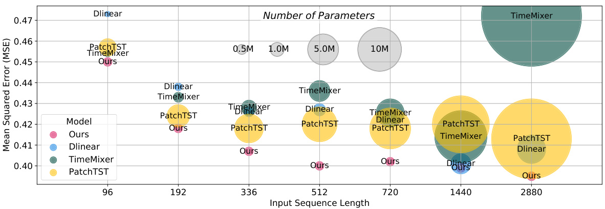
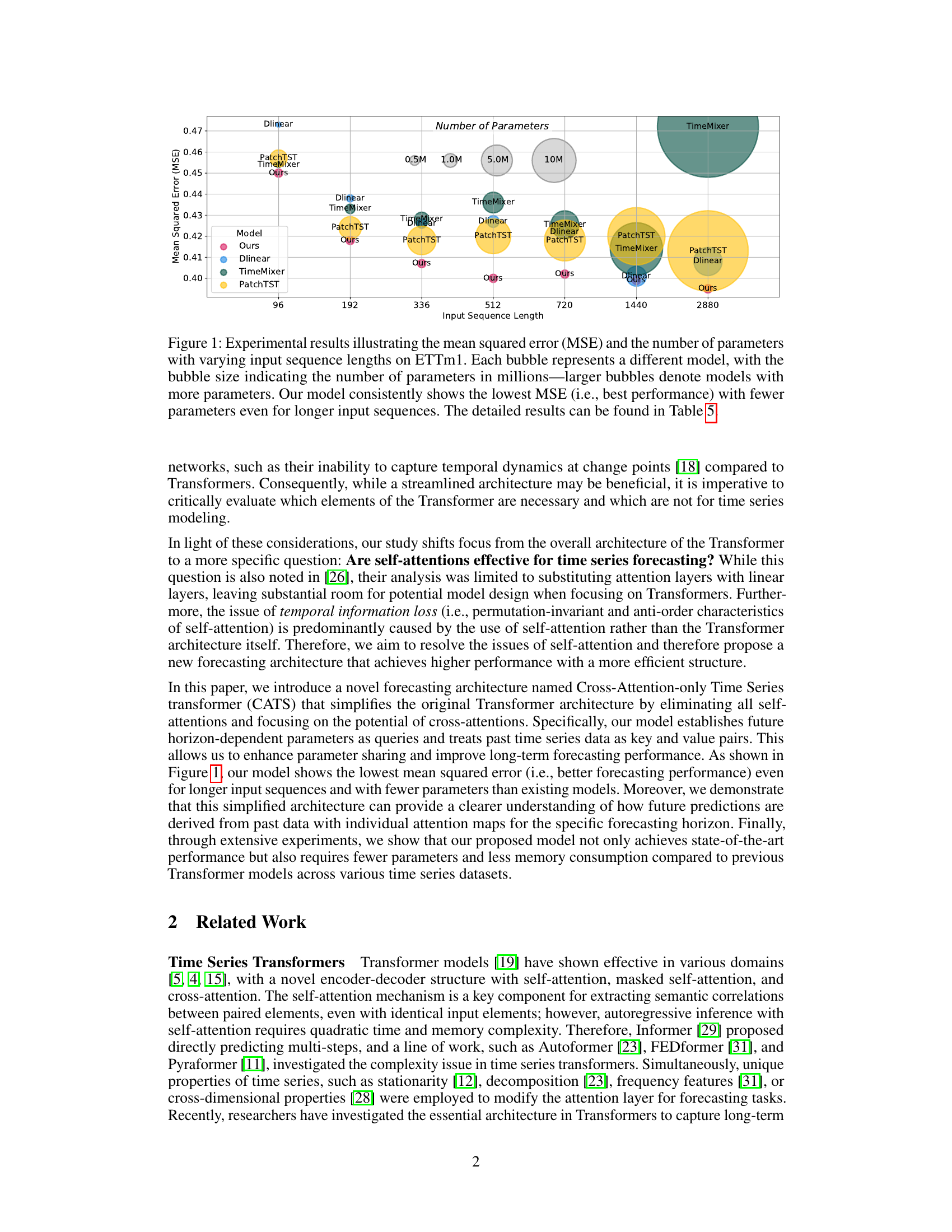
This figure shows the mean squared error (MSE) and the number of parameters (in millions) for different models on the ETTm1 dataset with various input sequence lengths. The size of each bubble corresponds to the number of parameters used. The model proposed in the paper (labeled ‘Ours’) consistently achieves the lowest MSE across all sequence lengths with the fewest number of parameters.
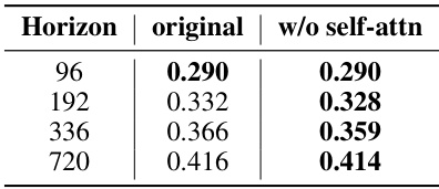
This table presents the mean squared error (MSE) results of the PatchTST model on the ETTm1 dataset, comparing the performance with and without self-attention for different forecasting horizons (96, 192, 336, and 720). It demonstrates the impact of removing self-attention on forecasting accuracy.
In-depth insights#
Self-Attn Reconsidered#
A section titled ‘Self-Attn Reconsidered’ in a research paper would likely delve into a critical re-evaluation of self-attention mechanisms, particularly within the context of time series forecasting. It would likely begin by acknowledging the widespread adoption of Transformers and their self-attention layers in various sequence modeling tasks, but then challenge the inherent assumptions of their universal effectiveness. The discussion might center on the computational cost associated with self-attention, which scales quadratically with sequence length, rendering it inefficient for very long time series. Furthermore, it could explore the potential limitations of self-attention in capturing temporal dynamics and long-range dependencies, possibly highlighting cases where simpler models outperform Transformers. A key part of this section would likely involve presenting empirical evidence, such as comparative results on benchmark datasets, to support claims of improved efficiency or accuracy through alternative approaches like cross-attention or entirely different architectures. Finally, ‘Self-Attn Reconsidered’ would likely conclude by offering new perspectives and potential directions for future research in time series forecasting, perhaps suggesting modifications to self-attention or proposing innovative alternatives.
CATS Architecture#
The CATS architecture presents a novel approach to time series forecasting by eliminating self-attention mechanisms entirely and relying solely on cross-attention. This design choice is motivated by concerns about the limitations of self-attention in capturing temporal dynamics and preserving temporal order in time series data, as highlighted in recent research. Cross-attention is strategically employed by using future horizons as queries and past time series data as keys and values. This setup allows for enhanced parameter sharing across different forecasting horizons, leading to efficiency gains in terms of the number of parameters and reduced computational cost. Furthermore, query-adaptive masking techniques are introduced to mitigate the risk of overfitting to the past data, ensuring that the model focuses sufficiently on the information relevant to each forecasting horizon. The combination of these innovations results in a simplified, computationally efficient, and more accurate forecasting architecture, offering a strong alternative to traditional Transformer-based models for various time series forecasting applications.
Long-Term Forecasting#
Long-term forecasting presents unique challenges due to the accumulation of errors over extended periods and the inherent complexities in capturing long-range dependencies within time series data. Traditional models often struggle with these challenges, especially when dealing with noisy or irregular data. This necessitates the development of specialized methods capable of handling the increased uncertainty and complexity. Transformer-based models, with their ability to learn intricate relationships between data points, have shown promise in long-term forecasting, but their computational costs and sensitivity to input sequence length remain significant limitations. The exploration of simpler architectures, such as the Cross-Attention-only Time Series Transformer (CATS), presents a compelling direction for improving efficiency and accuracy. This involves focusing on the essential components necessary for long-term prediction while optimizing for memory and computational requirements. Effective strategies for parameter sharing, query-adaptive masking, and efficient temporal encoding are crucial for achieving superior performance in this challenging domain. Furthermore, robustness to varying data patterns and lengths is paramount, requiring approaches that are both accurate and resilient to noise.
Efficiency Gains#
The concept of “Efficiency Gains” in the context of a machine learning research paper, particularly one focused on time series forecasting, likely revolves around reducing computational costs while maintaining or even improving accuracy. This could manifest in several ways: fewer model parameters leading to faster training and inference, reduced memory footprint enabling the use of larger datasets or longer sequences, or more efficient algorithms resulting in lower runtimes. A key aspect would be a comparison with existing state-of-the-art models, demonstrating a clear advantage in terms of resource usage. The discussion might also highlight the trade-offs involved, acknowledging that some efficiency gains may come at the cost of slight performance reductions. Furthermore, the analysis should extend beyond raw metrics to consider broader implications like scalability and accessibility, suggesting that the more efficient model is easier to deploy and use in diverse resource-constrained environments.
Future Work#
Future research directions stemming from this paper could explore several promising avenues. Extending CATS to handle multivariate time series with complex interdependencies is crucial, moving beyond the assumption of channel independence. Investigating the impact of different patching strategies and embedding techniques on long-term forecasting accuracy would further refine the model’s effectiveness. A comprehensive comparison of CATS against a broader range of state-of-the-art models, particularly those employing more sophisticated attention mechanisms or advanced architectures, is needed to solidify its position. Furthermore, exploring the potential of incorporating additional features or external knowledge into CATS, such as incorporating domain-specific information, could significantly enhance its predictive power. Finally, a deep dive into the theoretical underpinnings of CATS, including a formal analysis of its capacity to capture temporal dynamics, would bolster its foundational understanding and inform future improvements. This multifaceted approach to future work would solidify CATS’ place among time series forecasting models and pave the way for more accurate and efficient predictions across diverse applications.
More visual insights#
More on figures

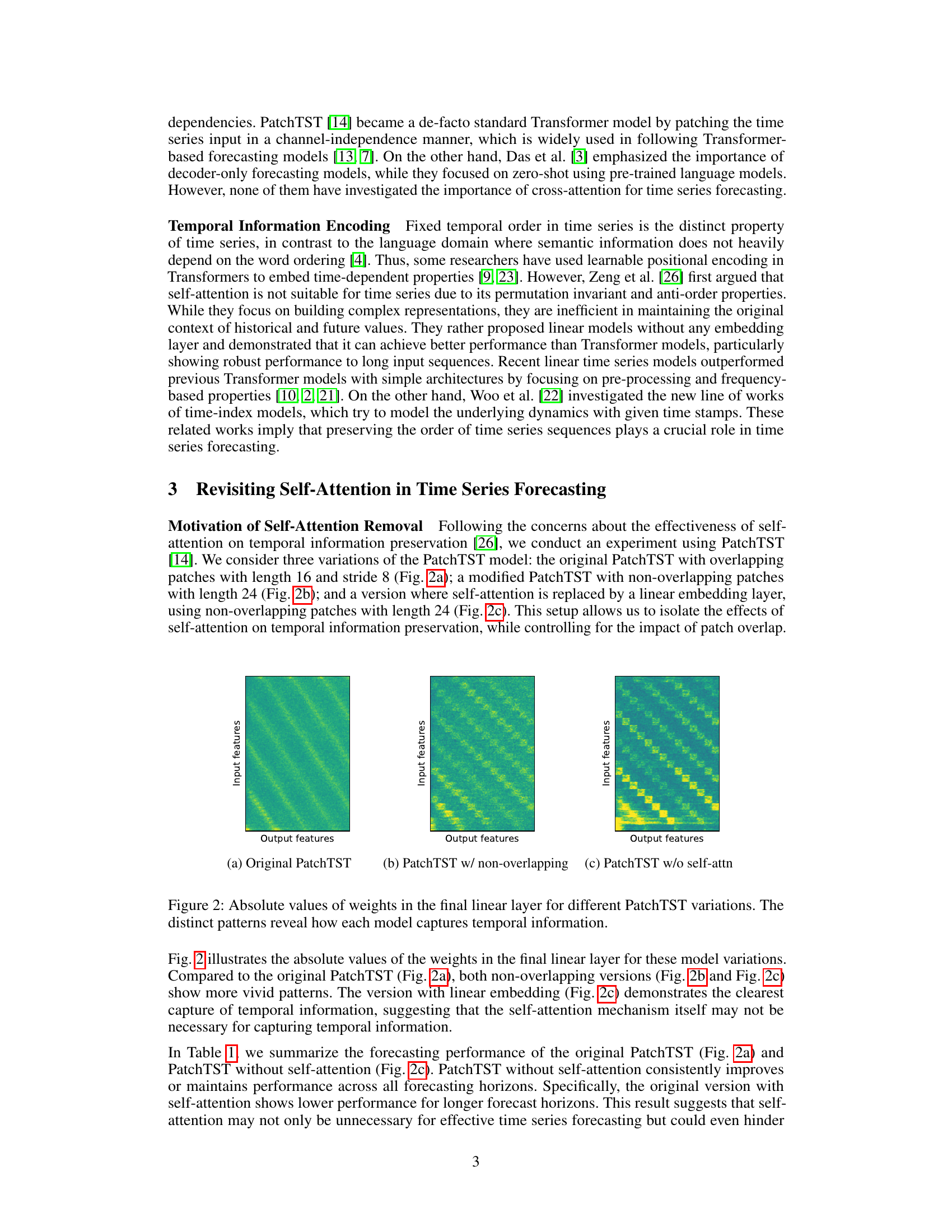
This figure shows the absolute values of weights in the final linear layer for three variations of the PatchTST model: (a) original PatchTST with overlapping patches, (b) PatchTST with non-overlapping patches, and (c) PatchTST with self-attention replaced by a linear embedding layer. The different patterns illustrate how effectively each model captures temporal information. The version with linear embedding shows the clearest capture, suggesting that self-attention is not necessary for this task.

This figure compares four different architectures for time series forecasting. (a) shows a standard Transformer architecture with both encoder and decoder, using self-attention and cross-attention mechanisms. (b) is a simplified encoder-only Transformer architecture, relying only on self-attention. (c) represents a linear model, which does not use any attention mechanism. (d) is the proposed CATS (Cross-Attention-only Time Series Transformer) architecture, which only uses cross-attention and eliminates self-attention.

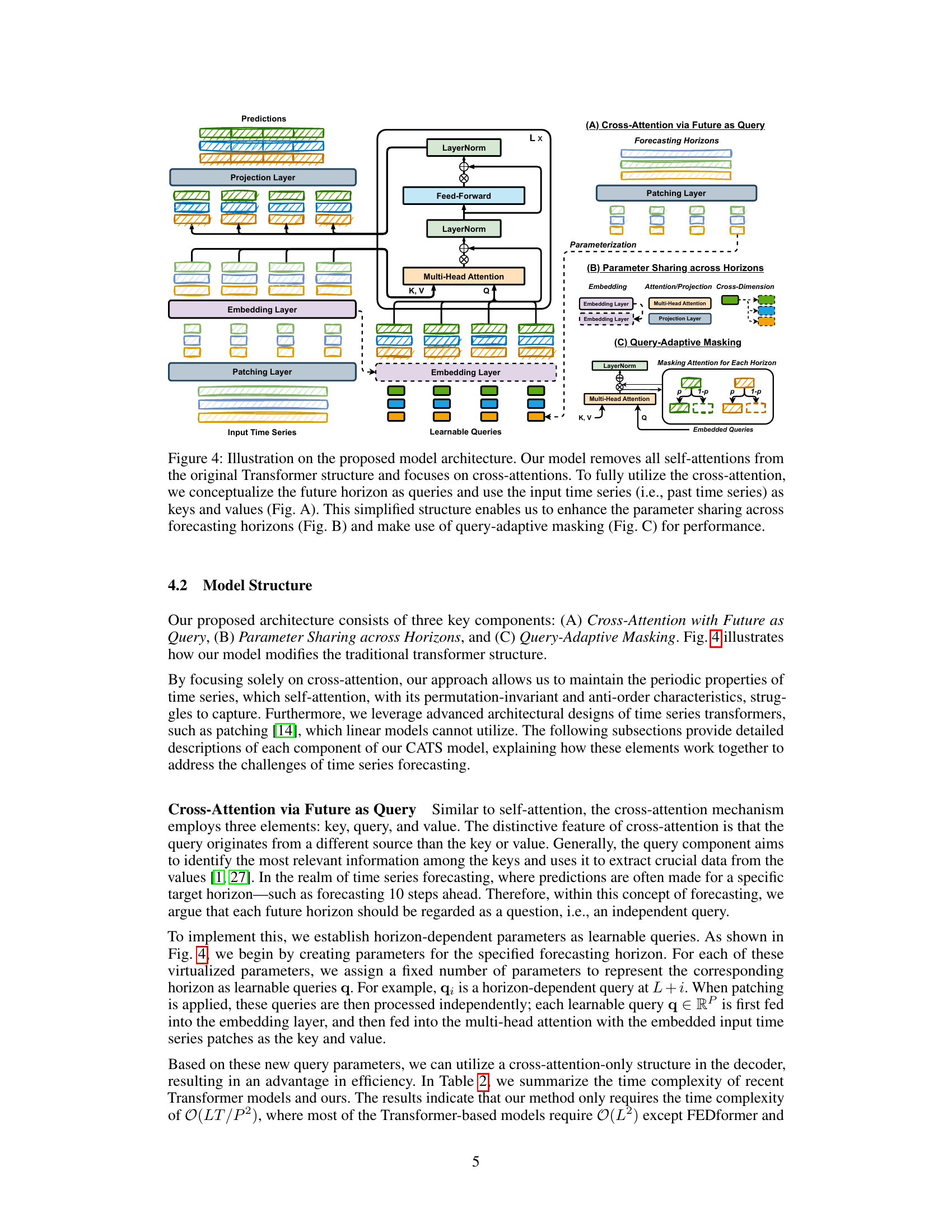
This figure illustrates the architecture of the proposed Cross-Attention-only Time Series Transformer (CATS) model. It highlights three key components: (A) Cross-Attention with Future as Query, (B) Parameter Sharing across Horizons, and (C) Query-Adaptive Masking. Panel A shows how future horizons are used as queries in the cross-attention mechanism, while past time series data serve as keys and values. Panel B demonstrates the parameter sharing strategy employed to enhance efficiency. Panel C details the query-adaptive masking technique used to improve performance by preventing access to irrelevant time series data for each horizon.

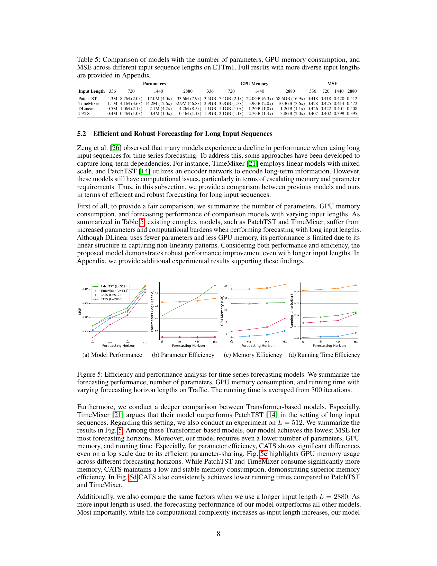
This figure presents a comparative analysis of various time series forecasting models, focusing on efficiency and performance across different forecasting horizons on the Traffic dataset. It shows four sub-figures: (a) Model Performance (MSE across different forecasting horizons), (b) Parameter Efficiency (number of parameters across horizons), (c) Memory Efficiency (GPU memory consumption across horizons), and (d) Running Time Efficiency (running time per iteration across horizons). The analysis reveals that the proposed CATS model demonstrates superior performance and efficiency compared to other models, especially for longer forecasting horizons.

The figure shows the cross-attention score maps (12 × 18) for two attention heads in the CATS model. Each map visualizes the attention weights between input and output patches, revealing how the model attends to different parts of the input sequence when making predictions. The patterns in the maps illustrate the model’s ability to capture both shock values and periodicities in the input time series data. Specifically, the periodic patterns in the attention weights reflect the model’s understanding of the temporal dependencies in the data, which is essential for accurate time series forecasting. The clear patterns in the attention weights show the model’s capacity to discern temporal structures in the input data and use that information effectively for prediction. The higher the value in the map, the stronger the attention between the corresponding input and output patches.

This figure visualizes the attention weights between input and output patches in the Cross-Attention-only Time Series Transformer (CATS) model. It shows how the model attends to different parts of the input sequence when making predictions. The distinct patterns reveal how the model captures temporal information and periodic patterns in time series data. Specifically, it highlights the model’s ability to identify and utilize periodic information for accurate forecasting. The clarity of the patterns in this figure contrasts with previous models and showcases the advantages of CATS.
This figure compares the performance of different time series forecasting models, including the proposed CATS model, on the ETTm1 dataset. It visualizes the mean squared error (MSE) achieved by each model against the number of parameters used. The size of each bubble corresponds to the number of parameters (in millions), allowing for a visual comparison of model complexity. The figure demonstrates that the CATS model consistently achieves the lowest MSE with a significantly smaller number of parameters, highlighting its superior performance and efficiency.
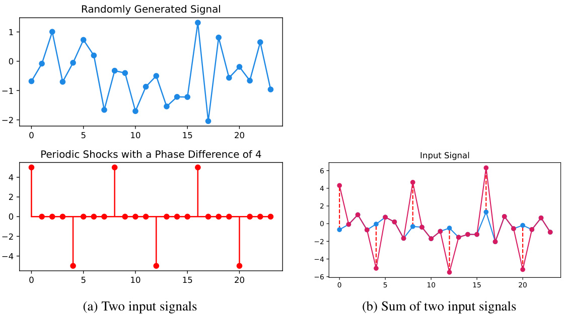
This figure visualizes the two synthetic input signals used in the toy experiment presented in Section 5.5 of the paper. The first signal is a randomly generated time series, illustrating the complexity and unpredictability of real-world data. The second signal is designed to incorporate a periodic shock component with a phase difference of 4, representing periodic patterns often found in real-world time-series such as electricity demand or weather data. The third subplot shows the combination of the two signals, designed to test the model’s ability to distinguish between noise and periodic patterns.

This figure shows the forecasting results of the proposed CATS model on the ETTm1 dataset. It highlights the model’s ability to capture temporal dependencies through cross-attention. Panel (a) presents the predicted and actual time series. Panel (b) displays a heatmap representing the average cross-attention scores across all attention heads and layers. The brighter the color, the higher the attention score, indicating stronger relationships between input and output patches. Panels (c) and (d) zoom into specific patches with the highest attention scores, demonstrating how CATS uses past data to predict future values, showcasing its understanding of temporal patterns.

This figure visualizes the attention weights between input and output patches in the CATS model. The heatmaps show the attention scores for two different attention heads. The distinct patterns reveal how the model captures temporal information and periodic patterns within the time series data, highlighting the effectiveness of cross-attention in this architecture.

This figure visualizes the forecasting results of the CATS model on the ETTm1 dataset, along with the averaged cross-attention score map. The score map highlights the attention weights assigned to different input patches during prediction. The figure also shows two example pairs of input and output patches with the highest attention weights. These visualizations illustrate how CATS leverages cross-attention to capture temporal dependencies and patterns in the time series data for accurate forecasting.

This figure shows the forecasting results, cross-attention score map, and patches with the highest attention scores for the ETTm1 dataset. The cross-attention score map visualizes the attention weights between input and output patches, highlighting the model’s ability to capture temporal dependencies and periodic patterns in the time series data. The patches with the highest scores further illustrate how the model focuses on specific parts of the time series for accurate predictions. This figure provides visual support for the model’s ability to effectively capture temporal patterns and improve prediction accuracy.

This figure visualizes the attention weights between input and output patches in the CATS model. The distinct patterns reveal how the model captures temporal information, particularly periodic patterns. The heatmap shows the attention scores for each pair of input and output patches, illustrating which input patches are most relevant to predicting each output patch’s value. High attention scores indicate a strong relationship between the corresponding input and output patches.

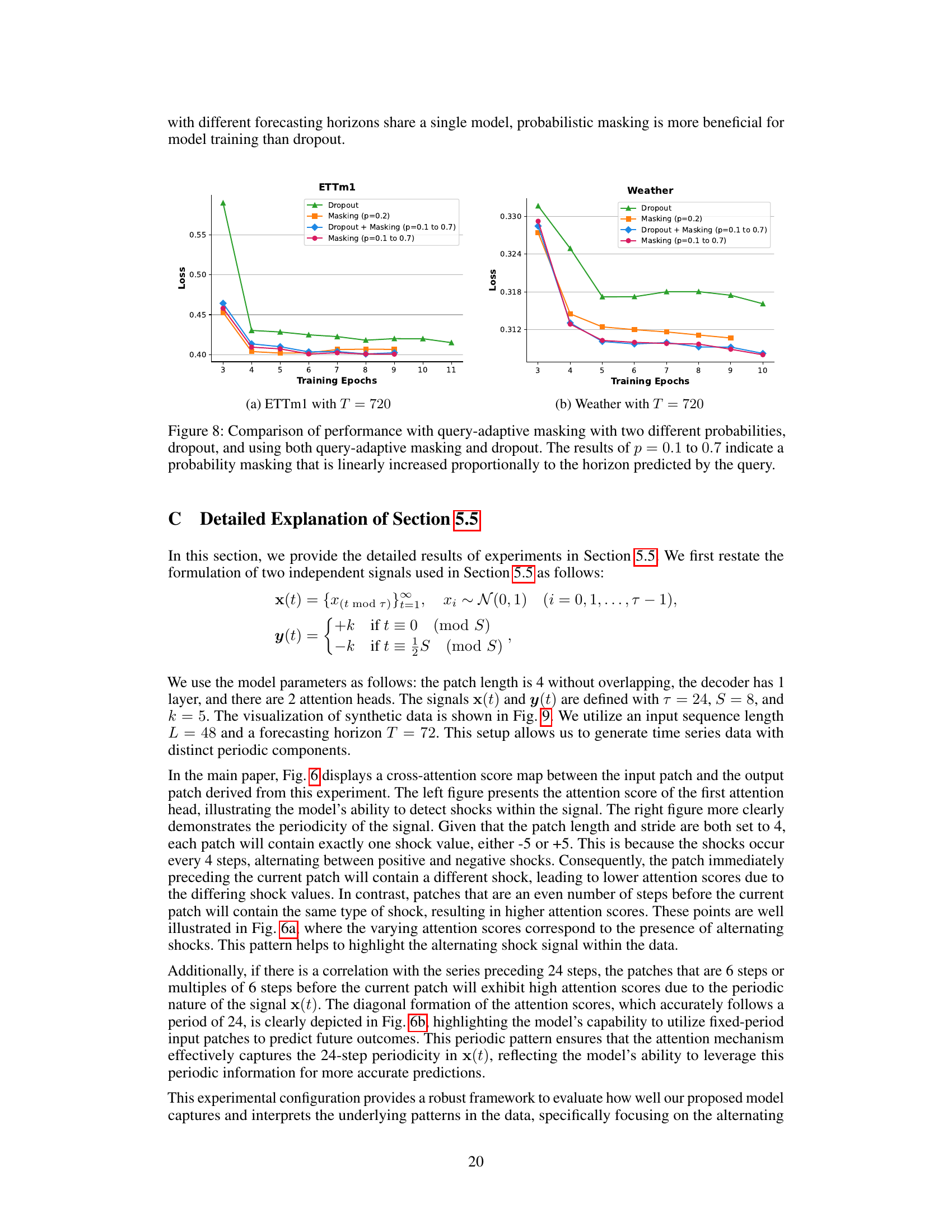
Figure 7 presents the forecasting results and cross-attention scores on the ETTm1 dataset, highlighting the model’s ability to capture temporal patterns. Subfigure (a) shows the forecasting results, comparing ground truth and model predictions. Subfigure (b) displays an averaged cross-attention score map, visualizing the attention weights between input and output patches. Subfigures (c) and (d) illustrate specific patch pairs with the highest attention weights, further demonstrating the model’s capacity to detect and utilize sequential patterns for forecasting.
More on tables

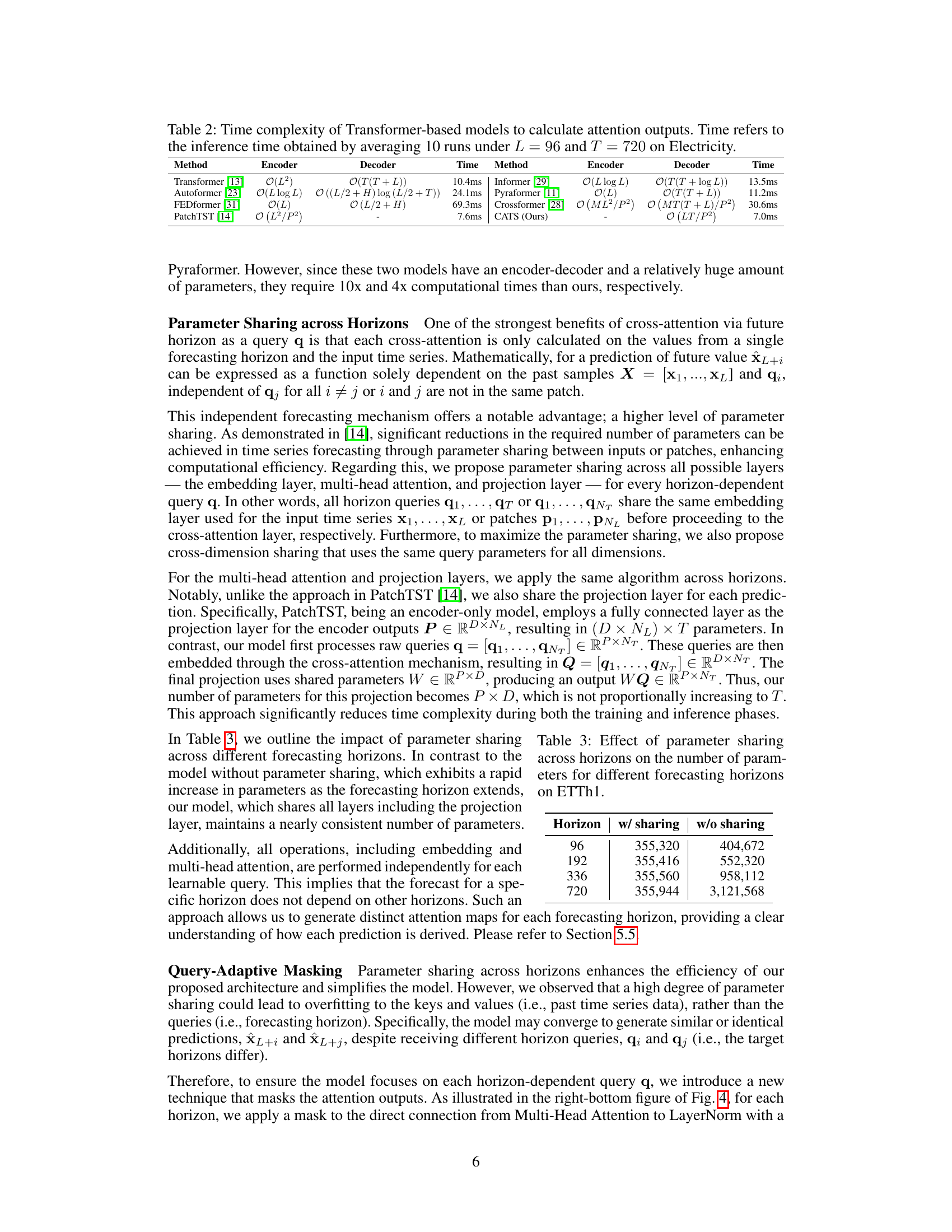
This table compares the time complexity of various Transformer-based models for calculating attention outputs. The time complexity is expressed using Big O notation, and the actual inference time (in milliseconds) is reported for an experiment with input sequence length L=96 and forecasting horizon T=720 on the Electricity dataset. The models included are Transformer, Informer, Autoformer, FEDformer, Pyraformer, Crossformer, PatchTST, and the authors’ proposed CATS model. The table highlights the significant efficiency gains achieved by the CATS model compared to other Transformer models.
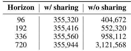
This table presents the number of parameters used in a model with and without parameter sharing across different forecasting horizons. The results are shown for the ETTh1 dataset. The table highlights how parameter sharing significantly reduces the number of parameters, particularly as the forecasting horizon increases.

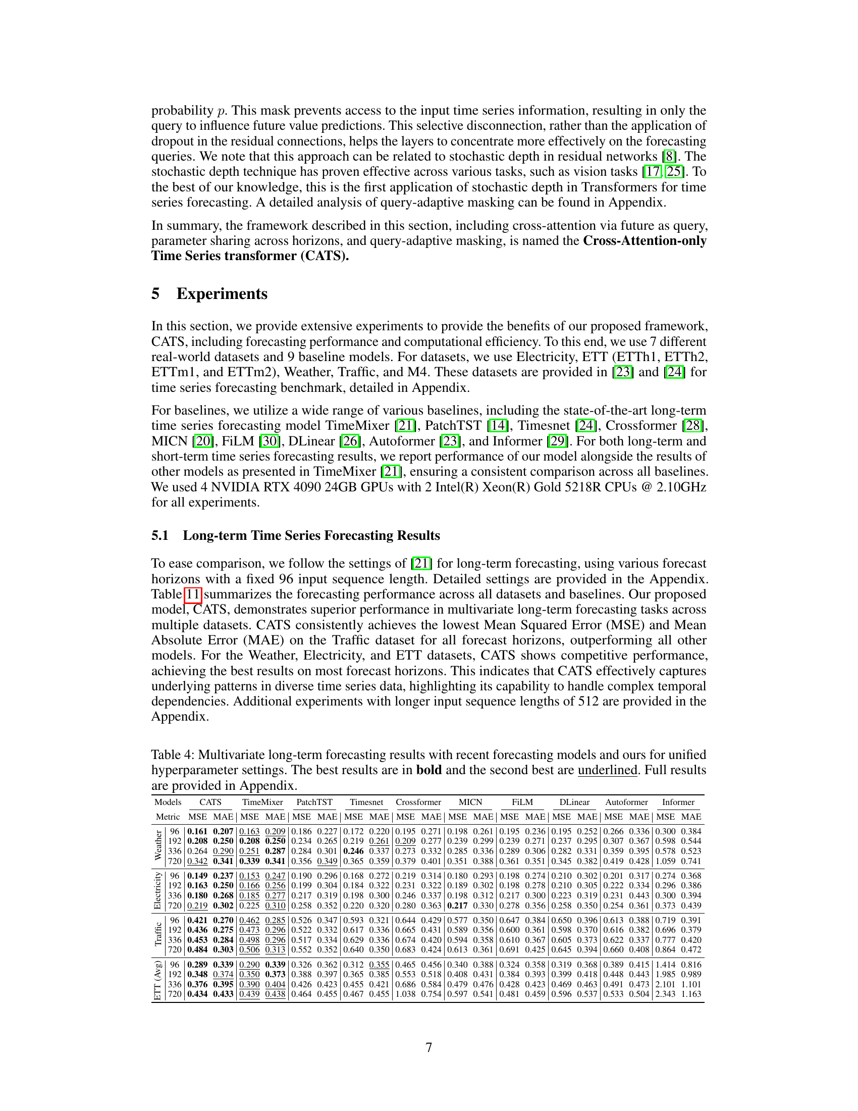
This table presents the results of multivariate long-term time series forecasting experiments using various models, including the proposed CATS model. The results are evaluated using Mean Squared Error (MSE) and Mean Absolute Error (MAE) metrics for different forecasting horizons (96, 192, 336, and 720) across four datasets (ETT, Traffic, Electricity, and Weather). The best performing model for each metric and horizon is highlighted in bold, and the second best is underlined. A more complete table with additional results is available in the appendix.

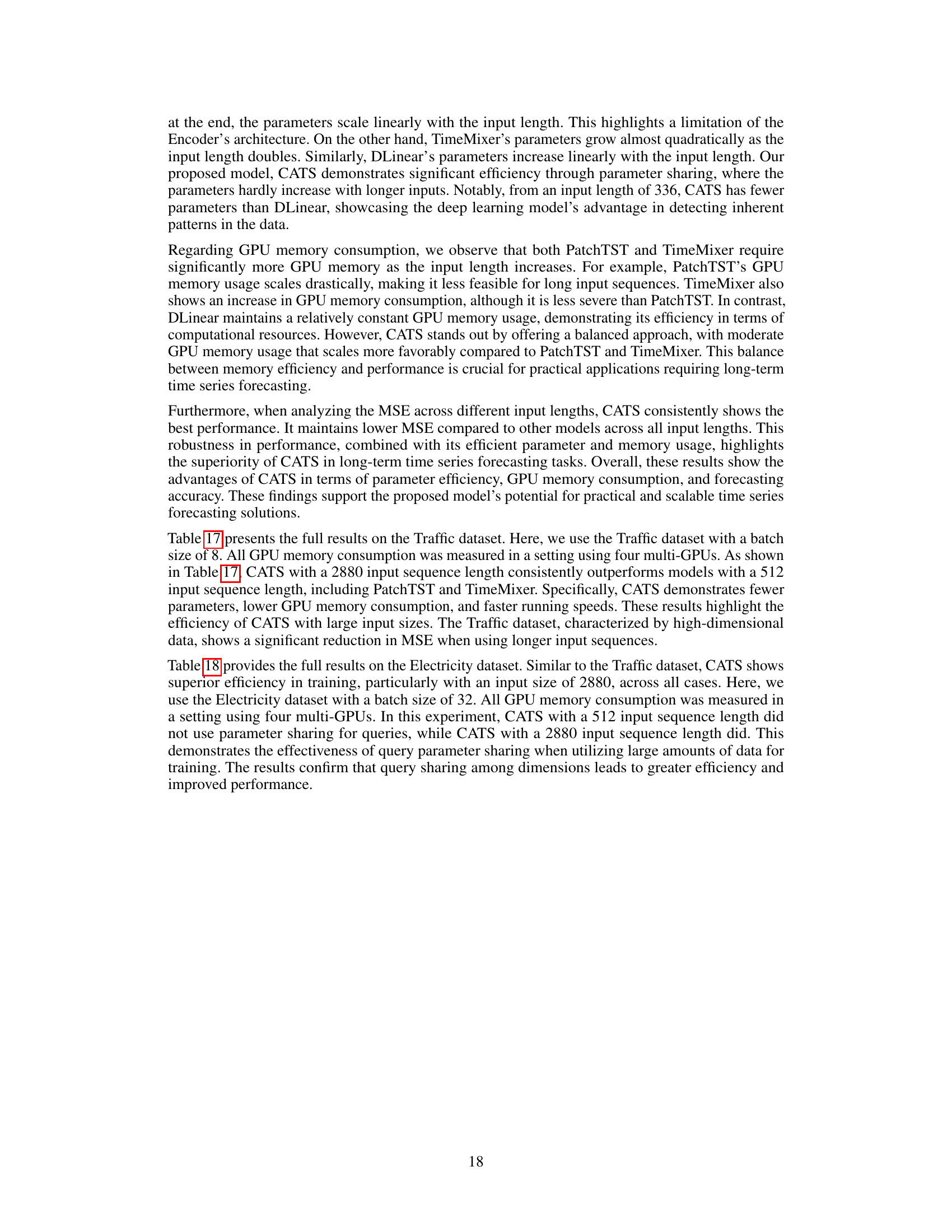
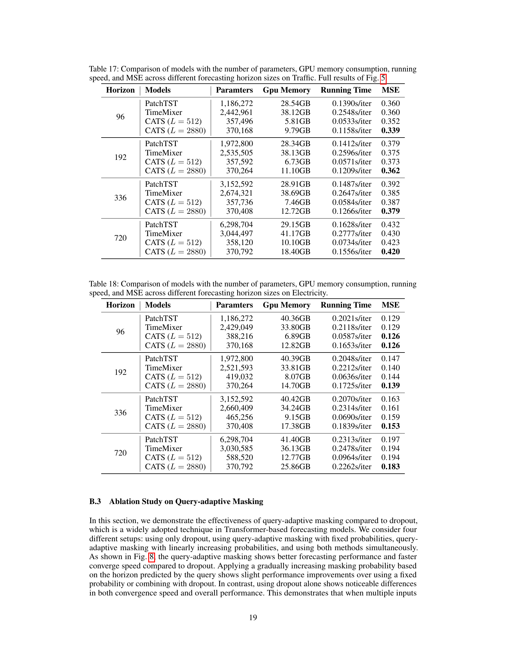
This table compares the performance of different time series forecasting models (PatchTST, TimeMixer, DLinear, and CATS) across various input sequence lengths (336, 720, 1440, and 2880) on the ETTm1 dataset. For each model and input length, the table shows the number of parameters (in millions), the GPU memory usage (in GB), and the mean squared error (MSE). The results highlight the impact of input sequence length on model complexity and performance. The full results with more diverse input lengths are available in the appendix.

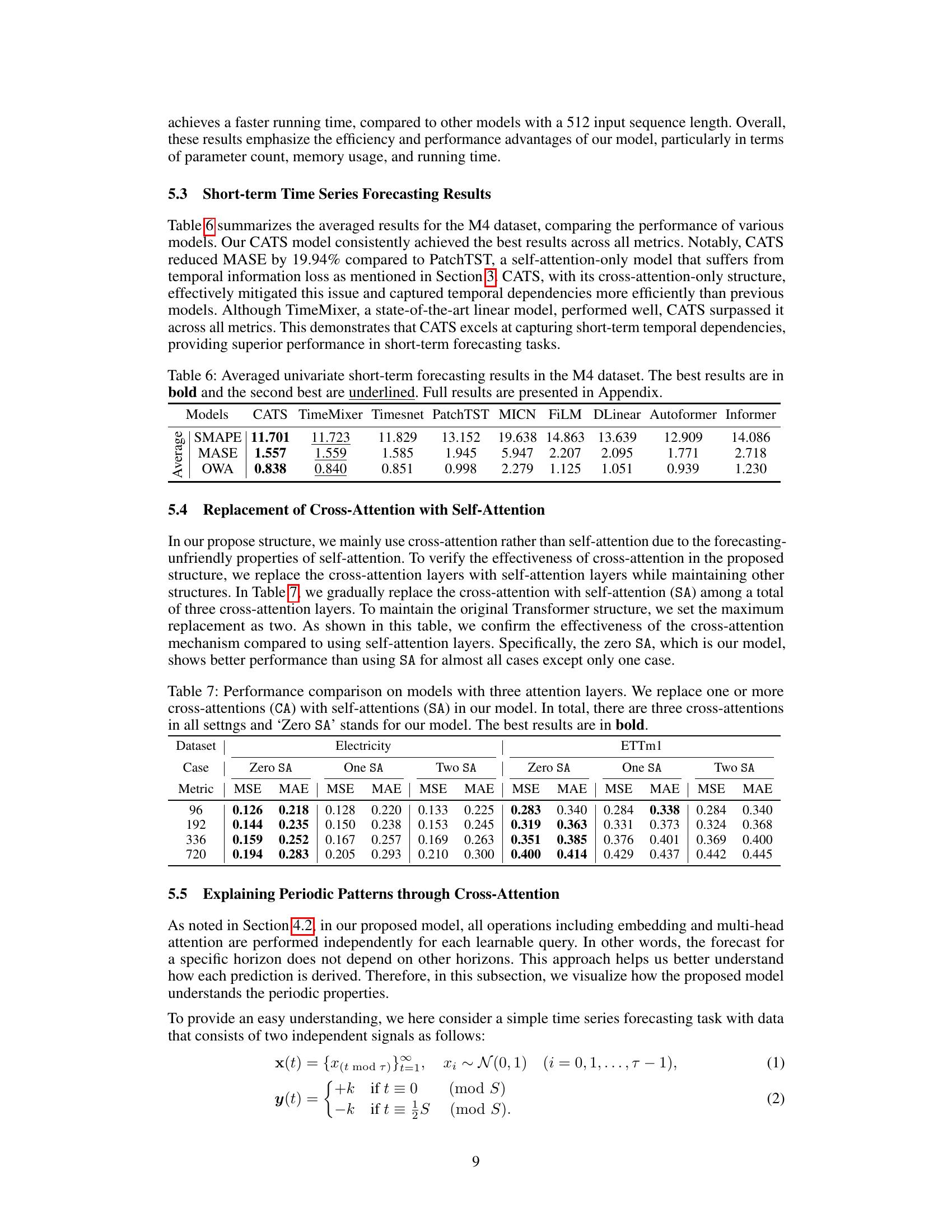
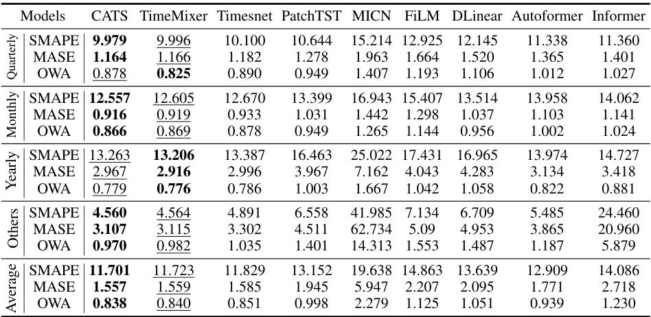
This table presents the average results of various models on the M4 dataset for short-term time series forecasting. The metrics used are SMAPE, MASE, and OWA. The best performing model for each metric is highlighted in bold, with the second-best underlined. Complete results can be found in the Appendix. This provides a comparison of CATS performance against several other state-of-the-art models in a commonly used benchmark for short-term time series prediction.

This table presents the results of an ablation study comparing the performance of the proposed model (CATS) with different numbers of self-attention layers. The ‘Zero SA’ row represents the original CATS model, which uses only cross-attention. The other rows show the performance when one or two of the cross-attention layers are replaced with self-attention layers. The table shows that the model performs best when only cross-attention is used (Zero SA).
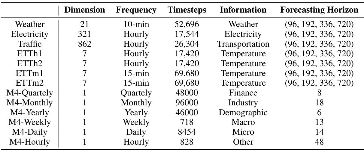
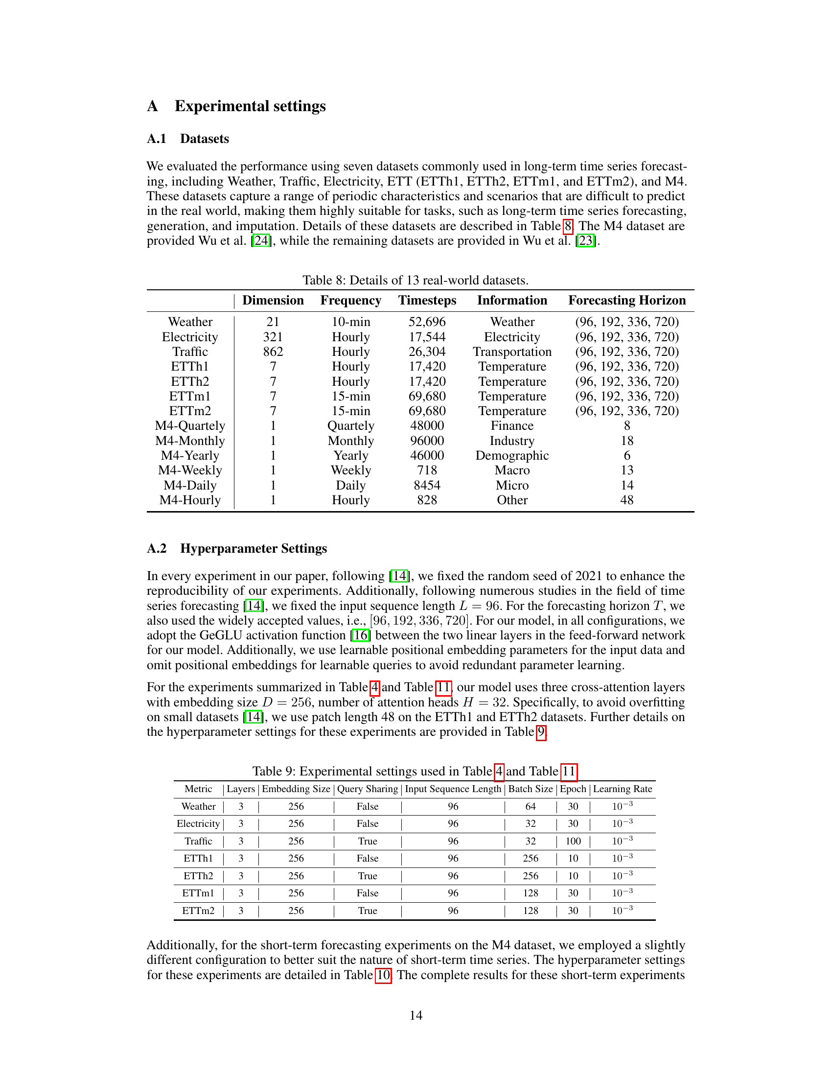
This table presents the details of thirteen real-world datasets used in the paper’s experiments on long-term time series forecasting. For each dataset, it lists the dimension (number of variables), frequency of data points (e.g., hourly, daily), total number of timesteps, the type of information contained, and the forecasting horizons used in the evaluations.

This table details the hyperparameter settings used for the experiments presented in Tables 4 and 11 of the paper. It specifies the number of layers, embedding size, whether query sharing was used, the input sequence length, batch size, number of epochs, and learning rate for each of the seven datasets used in the long-term forecasting experiments: Weather, Electricity, Traffic, ETTh1, ETTh2, ETTm1, and ETTm2. The settings were largely kept consistent to ensure fair comparison and reproducibility.

This table presents a comparison of the proposed CATS model’s performance against other state-of-the-art time series forecasting models on various datasets. The results are reported using two common metrics: Mean Squared Error (MSE) and Mean Absolute Error (MAE). The table shows the results for multiple forecasting horizons and highlights the superiority of the CATS model in many cases.
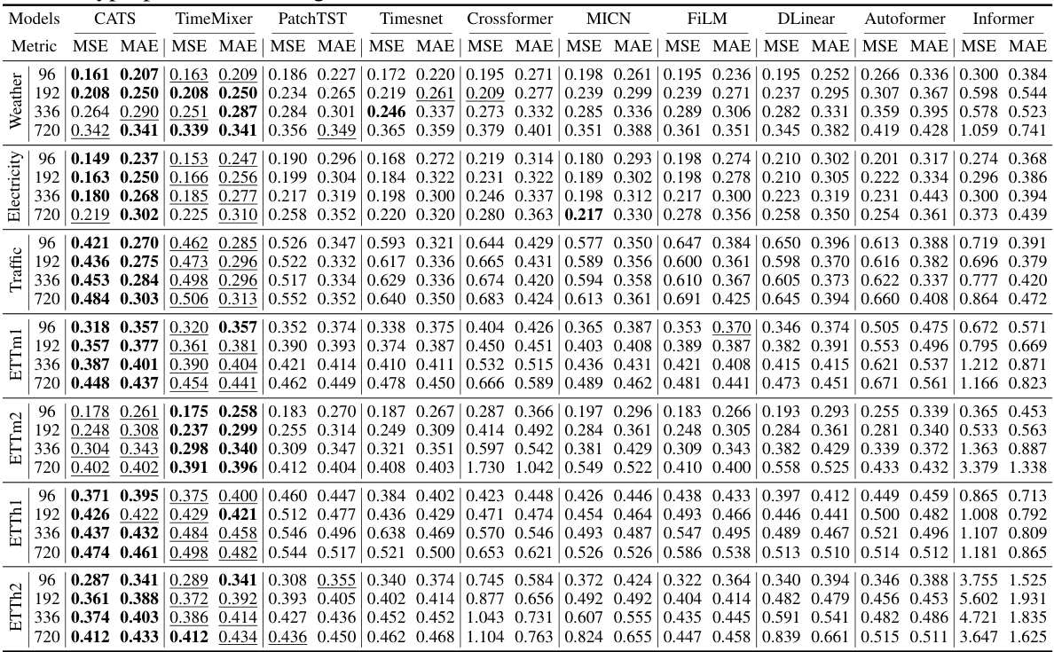
This table presents a comparison of the model’s performance (measured by MSE and MAE) on four different datasets (ETT, Traffic, Electricity, and Weather) across four different forecasting horizons (96, 192, 336, and 720). The results show that the proposed CATS model consistently achieves the lowest MSE and MAE, indicating superior performance compared to other state-of-the-art models for long-term forecasting tasks. The full results, including additional metrics, are available in the Appendix.
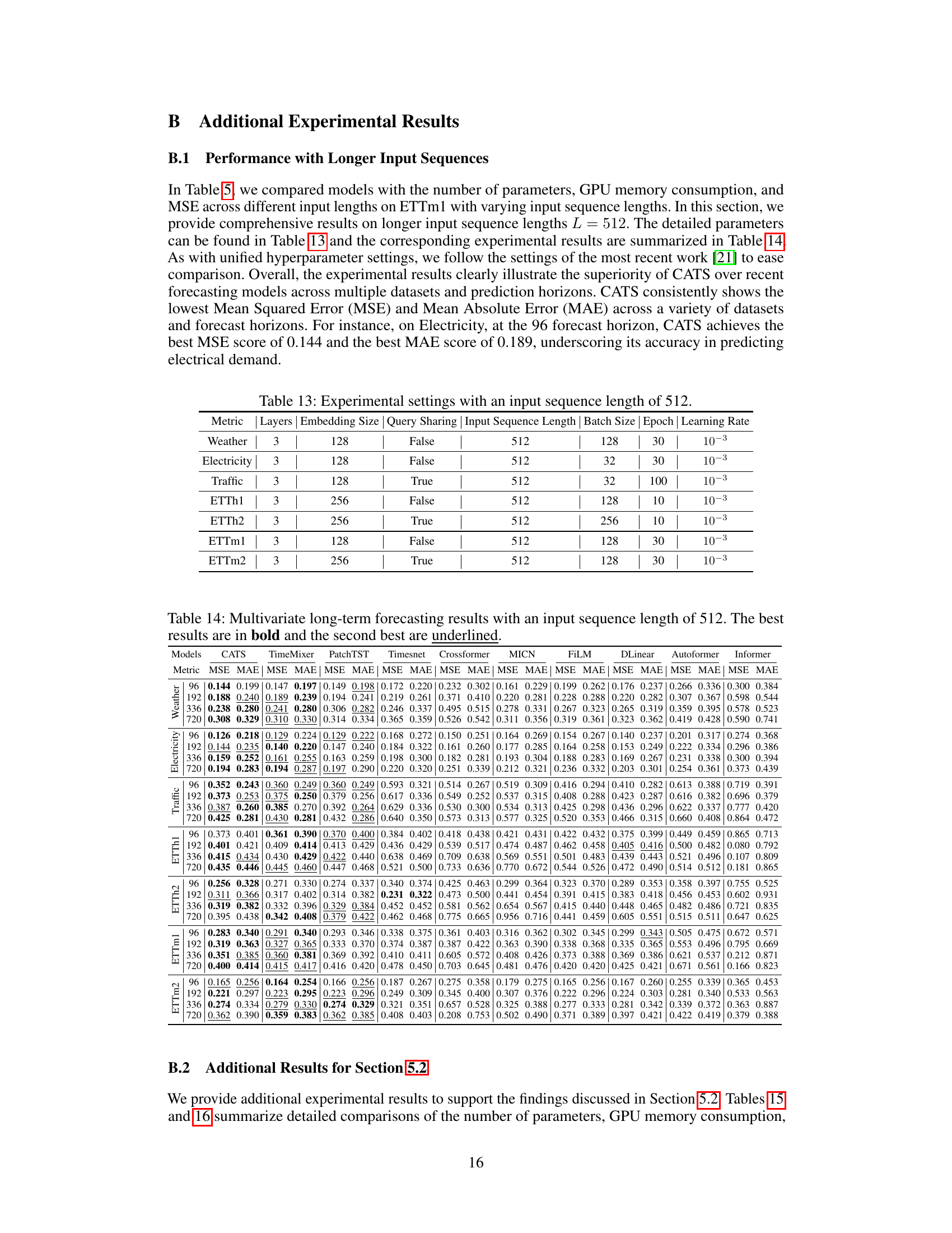
This table presents the mean squared error (MSE) and mean absolute error (MAE) for various long-term time series forecasting models on different datasets, including Electricity, Traffic, ETT (ETTh1, ETTh2, ETTm1, ETTm2) and Weather. The models compared include CATS (the proposed model), TimeMixer, PatchTST, Timesnet, Crossformer, MICN, FiLM, DLinear, Autoformer, and Informer. The table shows the performance of each model across different forecasting horizons (96, 192, 336, and 720) for each dataset. The best performance for each metric and horizon are highlighted in bold, and the second-best are underlined. The full results including additional metrics are given in the Appendix.

This table details the hyperparameters used in the experiments with an input sequence length of 512. It lists the specific settings for each of the seven datasets used in the paper’s long-term forecasting experiments (Weather, Electricity, Traffic, ETTh1, ETTh2, ETTm1, and ETTm2), including the number of layers, embedding size, query sharing, batch size, number of epochs, and learning rate. The variations in these settings reflect the diverse characteristics of the different datasets.
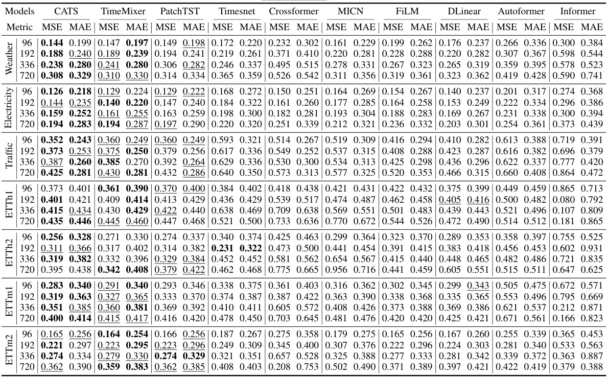
This table presents a comparison of the proposed CATS model’s performance against several state-of-the-art long-term forecasting models across various datasets and forecasting horizons. The metrics used for comparison are Mean Squared Error (MSE) and Mean Absolute Error (MAE). The best performing model for each metric and dataset is highlighted in bold, while the second-best is underlined. This provides a comprehensive overview of CATS’ performance relative to existing models in a long-term forecasting context.
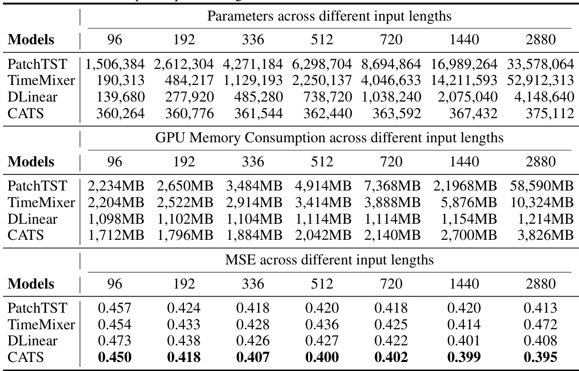
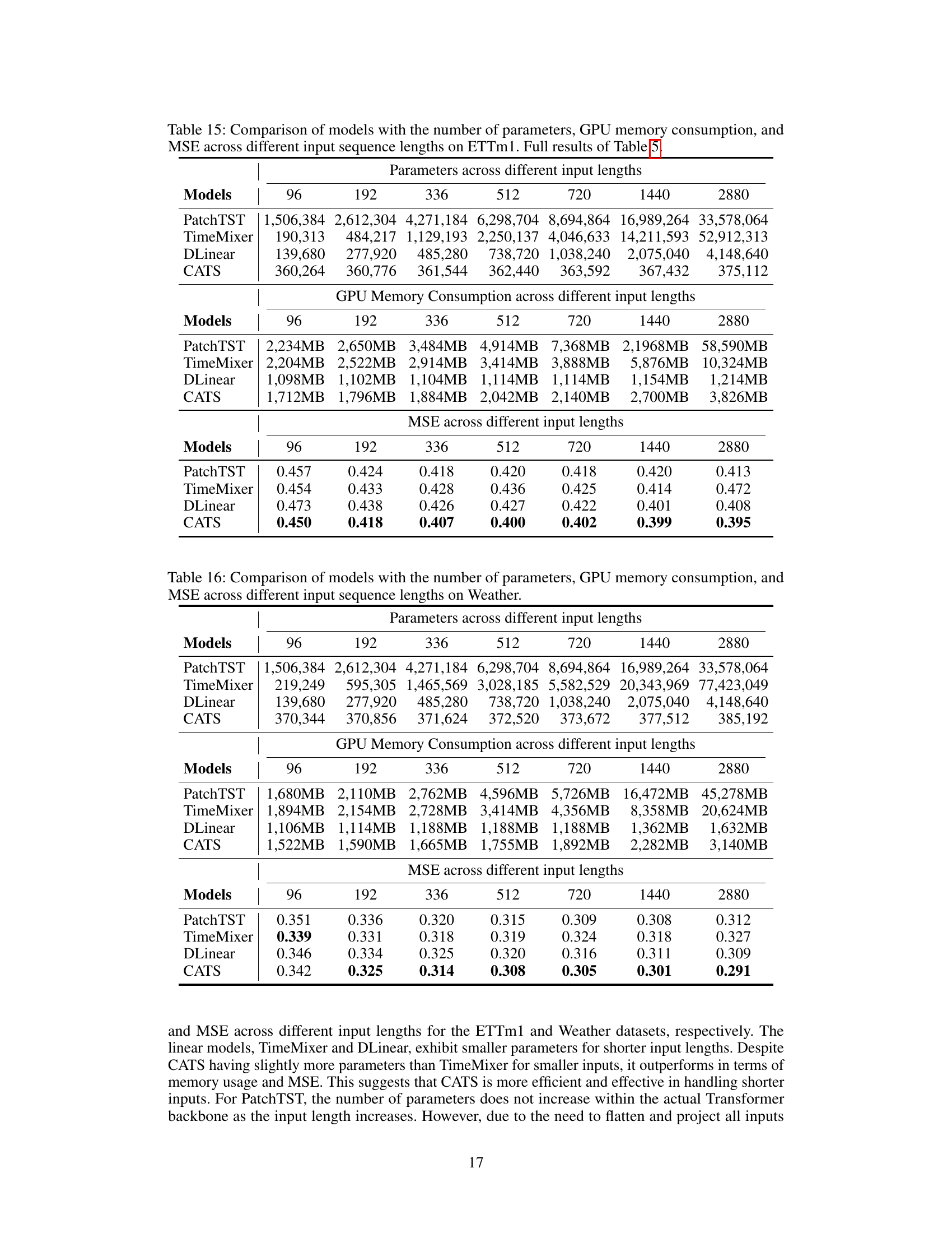
This table compares the performance of PatchTST, TimeMixer, DLinear, and CATS models across various input sequence lengths (96, 192, 336, 512, 720, 1440, 2880) on the ETTm1 dataset. For each model and sequence length, the number of parameters (in millions), GPU memory consumption (in MB), and Mean Squared Error (MSE) are reported. The table demonstrates how the model performance and resource requirements vary with the length of the input sequence, highlighting the efficiency of CATS in terms of parameter count and memory usage while maintaining competitive MSE values.

This table compares the performance of different time series forecasting models (PatchTST, TimeMixer, DLinear, and CATS) across various input sequence lengths (96, 192, 336, 512, 720, 1440, and 2880) on the ETTm1 dataset. It shows the number of parameters, GPU memory consumption, and mean squared error (MSE) for each model and input length. The goal is to demonstrate the efficiency and robustness of the proposed CATS model compared to existing models, particularly when dealing with longer input sequences.
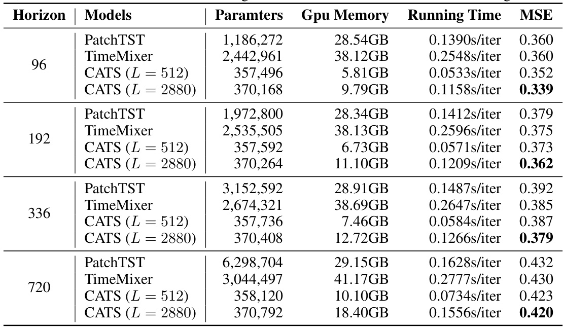
This table presents a comparison of the proposed CATS model with several state-of-the-art long-term time series forecasting models across multiple datasets and forecast horizons. The models were evaluated using a consistent set of hyperparameters to ensure fair comparison. The table shows Mean Squared Error (MSE) and Mean Absolute Error (MAE) for each model and dataset, highlighting CATS’ superior performance, particularly for longer horizons.
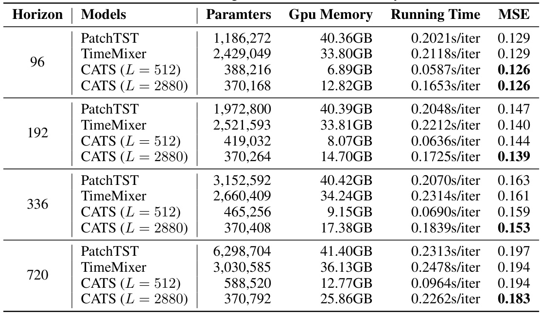
This table presents a comparison of the model’s performance in multivariate long-term forecasting. It shows the mean squared error (MSE) and mean absolute error (MAE) for various models (including the proposed CATS model) across different datasets and forecasting horizons. The best and second-best results for each metric are highlighted.
Full paper#

