↗ OpenReview ↗ NeurIPS Homepage ↗ Chat
TL;DR#
Many real-world applications involve time series forecasting where only partially observed data, solely focusing on endogenous variables, is insufficient for accurate predictions. Existing models either treat all variables equally (increasing complexity) or ignore exogenous information completely, leading to suboptimal results. This paper addresses this challenge by focusing on the practical scenario of forecasting with exogenous variables.
The proposed TimeXer method uses a canonical transformer architecture enhanced with new embedding layers to effectively combine endogenous and exogenous information. Patch-wise self-attention and variate-wise cross-attention mechanisms are employed simultaneously, allowing the model to learn both temporal dependencies within the endogenous series and the relationships between endogenous and exogenous variables. Experiments demonstrate that TimeXer achieves state-of-the-art results on twelve real-world benchmarks, showcasing its effectiveness, generality, and scalability in handling various data irregularities.
Key Takeaways#
Why does it matter?#
This paper is important because it presents TimeXer, a novel and effective approach to time series forecasting that significantly improves accuracy by incorporating exogenous variables. This addresses a critical limitation of existing methods and opens up new avenues for research in various domains requiring accurate predictions, such as meteorology, finance and traffic management. The model’s scalability and adaptability to real-world data irregularities make it particularly relevant to current research trends focusing on robust and generalizable forecasting techniques.
Visual Insights#

The figure on the left illustrates the concept of time series forecasting with exogenous variables. It shows how multiple external variables provide additional information to improve the accuracy of predicting the target variable (endogenous variable). The figure on the right presents a comparison of the performance of different time series forecasting models (TimeXer, Crossformer, DLinear, TIDE, iTransformer, PatchTST) on several real-world electricity price forecasting benchmarks, demonstrating the effectiveness of TimeXer.

This table compares various time series forecasting methods based on their capabilities in handling univariate and multivariate time series, and whether they explicitly model exogenous variables. The table uses checkmarks to indicate capabilities and a ‘◇’ to show methods that handle multivariate data but don’t directly model cross-variate dependencies. The table helps to position TimeXer within the existing landscape of forecasting methods.
In-depth insights#
TimeXer’s Design#
TimeXer’s design cleverly leverages the Transformer architecture, enhancing its capabilities for time series forecasting with exogenous variables. Patch-wise self-attention is applied to endogenous data, capturing temporal dependencies effectively. Variate-wise cross-attention between endogenous and exogenous variables ensures effective integration of external information. The use of learnable global endogenous tokens acts as a bridge, seamlessly incorporating exogenous information into the temporal dynamics of the endogenous series. This hybrid approach, combining patch-wise and variate-wise attention, allows TimeXer to handle the irregularities often present in real-world exogenous data, making it highly robust and adaptable. The simplicity and effectiveness of this design are key to its success, demonstrating how the core principles of the Transformer can be skillfully extended to solve complex forecasting problems.
Exogenous Handling#
The effective handling of exogenous variables is crucial for accurate time series forecasting, as these external factors often significantly influence the target variable. A robust approach should consider several key aspects. First, data preprocessing is essential to address issues like missing values, misaligned timestamps, and varying frequencies in exogenous data. Second, the method of integration is critical; simple concatenation may not capture complex interactions. More sophisticated methods, like embedding layers and attention mechanisms, are needed to effectively integrate exogenous information with endogenous data. Third, the model’s architecture must be designed to handle the diverse nature of exogenous inputs, possibly using specialized layers or modules to process different data types. Finally, model evaluation requires careful consideration of both endogenous and exogenous data, acknowledging the potential for biases and confounding factors. A comprehensive approach to exogenous variable handling can significantly improve the accuracy and reliability of time series forecasts.
Empirical Results#
An ‘Empirical Results’ section in a research paper would typically present quantitative findings that validate the study’s hypotheses. A strong section would begin by clearly stating the metrics used to evaluate performance (e.g., accuracy, precision, recall, F1-score, AUC, MSE). Then, it should present the results in a clear and concise manner, often using tables or figures to show the performance of the proposed method(s) compared to existing baselines. Statistical significance testing (e.g., t-tests, ANOVA, paired t-tests) should be applied where appropriate to demonstrate the reliability of any observed differences. The discussion should focus on the key trends, such as comparing the performance across different datasets or experimental settings, and highlight any unexpected or noteworthy findings. Crucially, a good section would not simply list the numbers but would also offer interpretations of the results in relation to the research questions and discuss any limitations of the study’s methodology. A robust empirical results section would thus provide compelling evidence for the study’s claims, enhancing the overall impact and credibility of the paper.
Ablation Study#
An ablation study systematically removes or alters components of a model to understand their individual contributions. In the context of a time series forecasting model with exogenous variables, this might involve removing the exogenous variable input, different embedding techniques, the cross-attention mechanism, or the global endogenous token. Analyzing the impact of each ablation on forecast accuracy reveals the importance of each component. For example, removing the exogenous variables entirely might lead to a significant drop in accuracy, highlighting their value. Similarly, disabling the cross-attention could indicate whether effectively integrating endogenous and exogenous information is crucial. Careful analysis helps optimize model architecture and identify critical features, ultimately leading to a more accurate and efficient forecasting system. The results are expected to highlight the relative importance of various model components and justify design decisions, demonstrating a robust and well-understood model architecture. Furthermore, comparing the impact of different embedding strategies will showcase the efficacy of the chosen approach.
Future Work#
Future work for TimeXer could explore several promising avenues. Extending TimeXer’s capabilities to handle high-dimensional and irregular time series data is crucial for broader real-world applicability. Investigating more sophisticated attention mechanisms, such as sparse attention or linear attention, could improve computational efficiency, particularly for long sequences. Incorporating advanced imputation techniques for missing data in exogenous and endogenous variables would enhance robustness and accuracy. A thorough investigation into the explainability of TimeXer’s predictions is needed, potentially through techniques like attention visualization or SHAP values, to increase trust and facilitate decision-making. Finally, exploring applications in other domains besides electricity and weather forecasting, such as finance, healthcare, and transportation, would showcase TimeXer’s generalizability and impact. Developing a comprehensive benchmark specifically for time series forecasting with exogenous variables would benefit the field significantly.
More visual insights#
More on figures
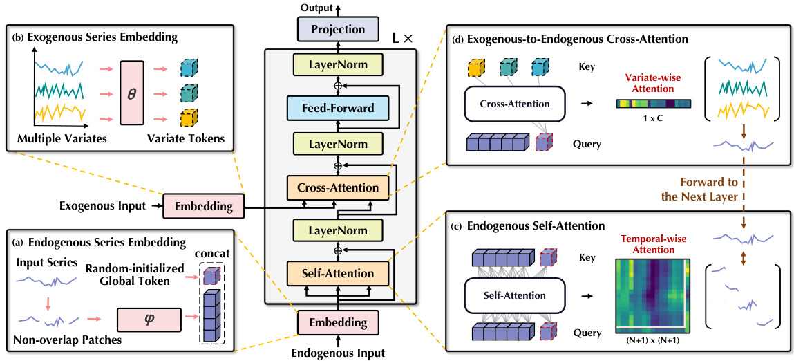
This figure illustrates the architecture of the TimeXer model. It shows how the model processes both endogenous (target) and exogenous (auxiliary) time series data. The endogenous series is first embedded into patch-wise temporal tokens and a global token. The exogenous series are embedded into variate-wise tokens. Self-attention is applied within the endogenous tokens to capture temporal dependencies. Cross-attention is then used to integrate the exogenous information with the endogenous information, facilitated by the global token. This combined information is then fed into subsequent layers for prediction.

This figure illustrates the TimeXer model architecture, showing how it processes endogenous and exogenous time series data. The endogenous series is split into patches, each represented by a token, and a global token summarizes the entire series. Exogenous series are each represented by a single variate token. Self-attention operates within the endogenous tokens, and cross-attention integrates information between the endogenous and exogenous tokens. The global endogenous token acts as a bridge between these two types of information.

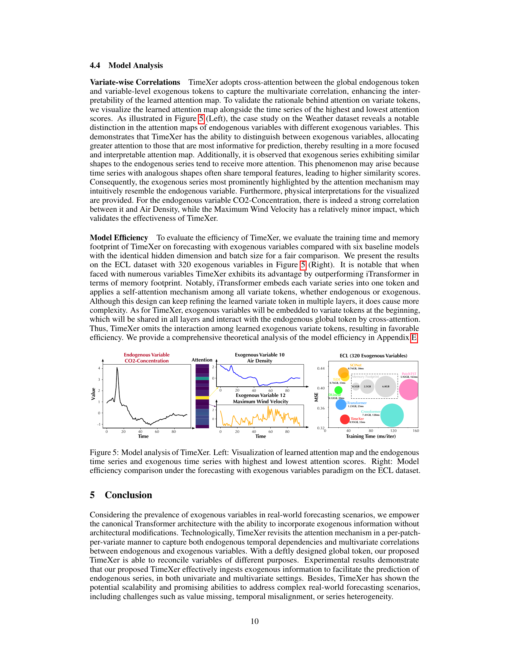
This figure demonstrates TimeXer’s performance on a large-scale weather forecasting task. The left panel shows a world map highlighting the locations of weather stations (endogenous variable) and their surrounding 3x3 grid areas (exogenous variables). Each grid provides four meteorological features (temperature, pressure, u-component of wind, v-component of wind). The right panel presents a bar chart comparing the Mean Squared Error (MSE) achieved by TimeXer against several other state-of-the-art forecasting models, illustrating TimeXer’s superior performance.

This figure illustrates the architecture of TimeXer, a novel approach for time series forecasting with exogenous variables. It shows how TimeXer uses different embedding strategies for endogenous and exogenous variables, employing patch-wise self-attention and variate-wise cross-attention mechanisms. The global endogenous token acts as a bridge, integrating exogenous information into the endogenous temporal patches. The figure is divided into four parts, showing (a) endogenous embedding, (b) exogenous embedding, (c) endogenous self-attention, and (d) exogenous-to-endogenous cross-attention.
This figure illustrates the architecture of the TimeXer model. It breaks down the process into four key stages: (a) Endogenous Embedding: The model processes the endogenous (target) time series by dividing it into patches and creating a token representation for each patch. A separate global token is also created to represent the entire endogenous series. (b) Exogenous Embedding: Exogenous (external) time series are processed, each series creating a single variate-level token representation. (c) Endogenous Self-Attention: Self-attention mechanisms operate on the patch tokens and the global token to capture temporal dependencies within the target time series. (d) Exogenous-to-Endogenous Cross-Attention: Cross-attention links the endogenous tokens with the exogenous tokens, allowing the model to integrate external information into the forecasting process.

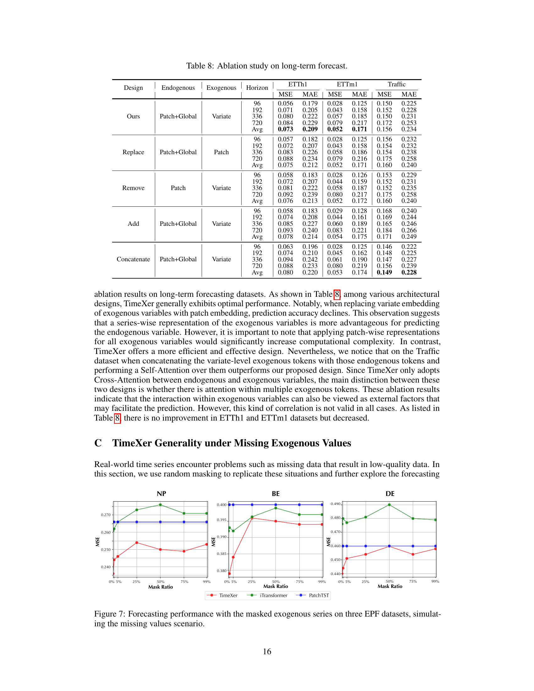
This figure showcases the impact of missing exogenous data on forecasting accuracy. It compares TimeXer, iTransformer, and PatchTST across three datasets (NP, BE, DE) at various levels of missing data (mask ratios). The results show the robustness or sensitivity of each model to missing exogenous information. The x-axis represents the percentage of missing exogenous data, while the y-axis shows the Mean Squared Error (MSE), a measure of prediction accuracy.
This figure illustrates the architecture of the TimeXer model, highlighting its key components and how they interact. It shows how endogenous and exogenous variables are processed separately and combined to enhance forecasting accuracy. The endogenous variable is split into patches which are processed via self-attention. Exogenous variables are represented by variate tokens. Global tokens bridge the information between the exogenous and endogenous components. Finally, cross-attention is used to integrate information between exogenous and endogenous series.
This figure illustrates the TimeXer model architecture, showcasing how it handles endogenous and exogenous variables. The endogenous variable is processed into multiple temporal tokens (patches) and a single global token which then undergoes self-attention. Each exogenous variable is represented as a variate token. Cross-attention combines the endogenous and exogenous information to improve forecasting accuracy.

This figure illustrates the architecture of the TimeXer model, highlighting the different embedding strategies and attention mechanisms used for endogenous and exogenous variables. It shows how the model processes the input time series data: (a) Endogenous data is split into patches, which are then embedded into temporal tokens, with a separate global token learned for the entire series. (b) Exogenous variables are represented by variate tokens. (c) Self-attention operates within the endogenous series to capture temporal relationships. (d) Cross-attention combines the endogenous and exogenous information, enabling the model to leverage exogenous information for improved prediction of the endogenous variable.

This figure illustrates the architecture of TimeXer, a novel approach for time series forecasting with exogenous variables. It shows the different embedding strategies used for endogenous (patch-wise) and exogenous (variate-wise) variables, and how self-attention and cross-attention mechanisms are used to capture dependencies within and between these variables. A key component is the inclusion of a learnable global token to bridge between endogenous and exogenous information.
This figure illustrates the TimeXer model architecture, highlighting the different embedding strategies used for endogenous and exogenous variables. Endogenous variables are processed using patch-wise self-attention and global endogenous tokens to capture temporal dependencies. Exogenous variables are processed using variate-wise cross-attention with the global endogenous tokens. This design allows TimeXer to effectively integrate both endogenous and exogenous information to enhance forecasting accuracy.
This figure illustrates the architecture of the TimeXer model. It shows how the model processes both endogenous (target) and exogenous (external) variables. The endogenous variables are embedded into multiple temporal tokens and a global token, enabling the capture of temporal dependencies using self-attention. Exogenous variables are represented as variate tokens that interact with the endogenous tokens and global token via cross-attention to incorporate external information. This combined approach allows the model to handle both internal temporal dynamics and the influence of external factors.

This figure illustrates the architecture of the TimeXer model, highlighting its key components. The model takes both endogenous (target) and exogenous (auxiliary) time series as input. Endogenous time series are embedded into multiple temporal tokens representing different segments, along with a global token to represent overall series information. Exogenous variables are each embedded into a single variate token. The model uses self-attention within endogenous tokens (temporal dependencies) and cross-attention between endogenous and exogenous tokens (integrating external information).
More on tables

This table presents a comprehensive comparison of the model’s performance (measured by MSE and MAE) on five different short-term electricity price forecasting datasets. The results are compared against nine state-of-the-art baseline models, highlighting TimeXer’s superior performance and consistency across various datasets. The standard protocol for short-term forecasting (input length=168, prediction length=24) is used for all models.

This table compares various time series forecasting models based on their capabilities, specifically focusing on whether they handle univariate or multivariate time series and if they explicitly model the cross-variate dependencies. The table uses a shorthand notation to represent the model’s capabilities, indicating whether they support univariate forecasting, multivariate forecasting, and forecasting with exogenous variables.

This table presents the ablation study results on the short-term electricity price forecasting task using the EPF dataset. It shows the impact of different design choices on the model’s performance, specifically focusing on the components of the endogenous and exogenous variable embeddings and the cross-attention mechanism. The rows represent different configurations, including removing or replacing certain components or using concatenation methods. The columns represent the performance metrics for various datasets (NP, PJM, BE, FR, DE), including Mean Squared Error (MSE) and Mean Absolute Error (MAE). The results highlight the contribution of each design element in the TimeXer model.

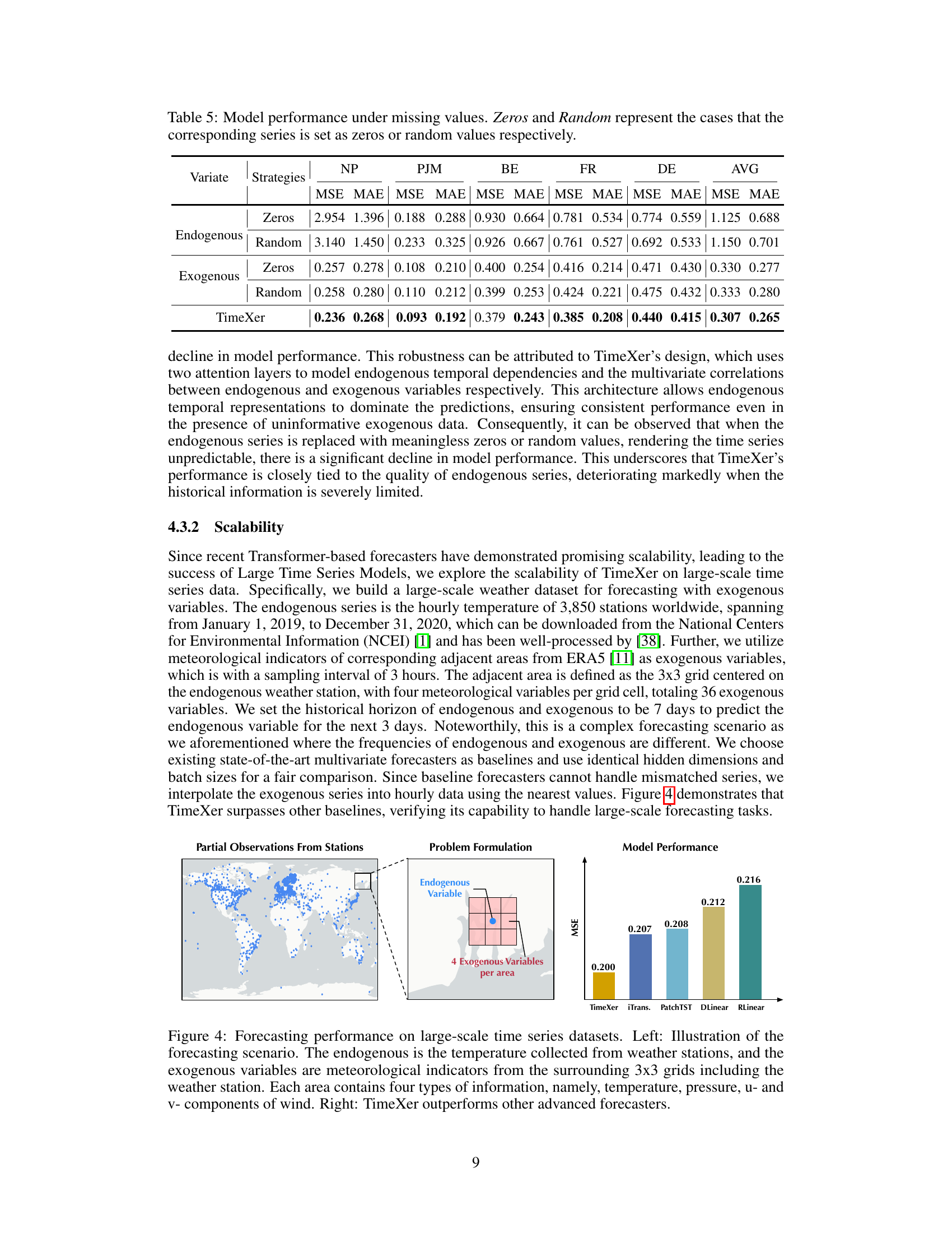
This table presents the results of an ablation study evaluating TimeXer’s robustness to missing data in exogenous variables. Two strategies were used to simulate missing data: filling the missing values with zeros or with random numbers. The table shows the Mean Squared Error (MSE) and Mean Absolute Error (MAE) for each dataset (NP, PJM, BE, FR, DE) and the average across all datasets (AVG) for each strategy applied to endogenous and exogenous variables. It demonstrates the impact of missing data on forecasting accuracy. The model performs best when all the data is complete, indicating that accurate information is important for proper predictions.

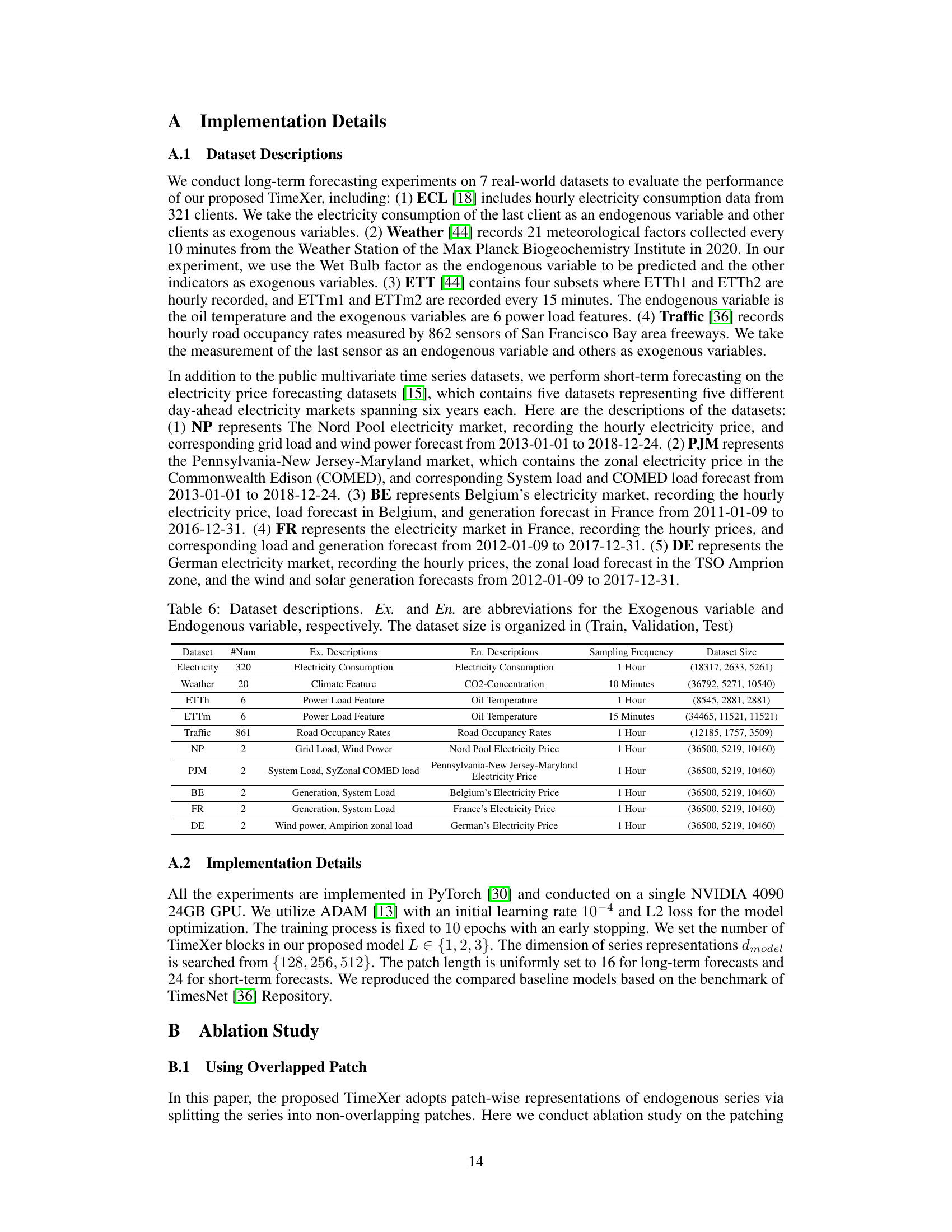
This table lists the characteristics of the seven datasets used in the paper’s experiments. For each dataset, it provides the name, number of exogenous and endogenous variables, sampling frequency, and the size of the training, validation, and test sets.

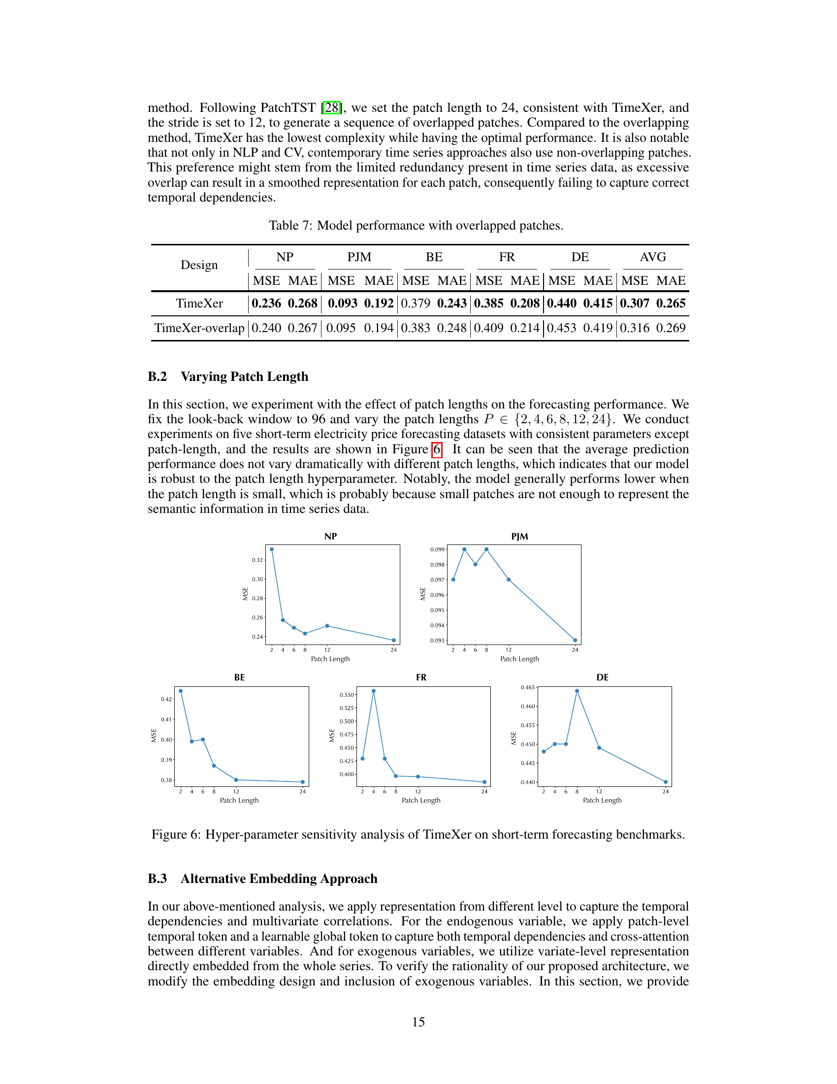
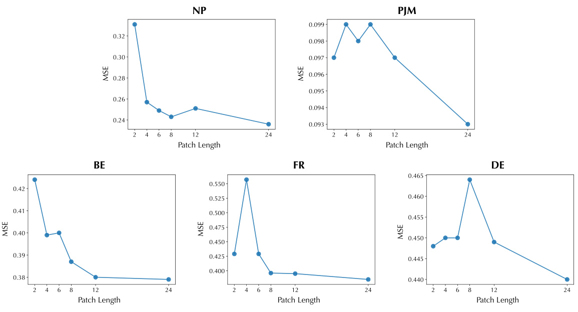
This table presents the performance comparison between TimeXer and TimeXer-overlap on five electricity price forecasting datasets. TimeXer-overlap uses overlapped patches, while TimeXer uses non-overlapping patches. The metrics used are MSE (Mean Squared Error) and MAE (Mean Absolute Error) for each dataset, along with an average across all five datasets. The results show that TimeXer achieves slightly better results than TimeXer-overlap in terms of both MSE and MAE. This suggests that the non-overlapping patch approach is more effective in this specific task.
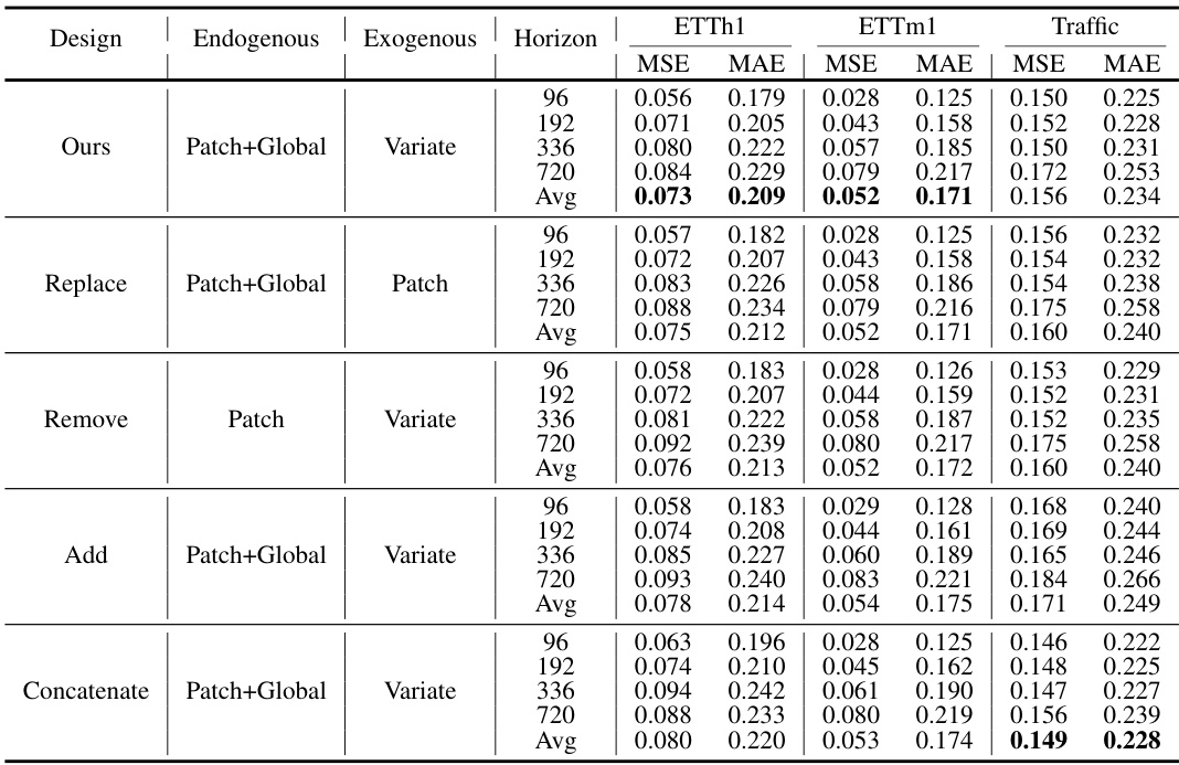
This table presents the ablation study results on long-term forecasting using different architectural designs of TimeXer. It compares the performance (MSE and MAE) of TimeXer with variations in the endogenous and exogenous variable embeddings. Specifically, it shows the effects of replacing, removing, adding, or concatenating the different types of tokens (patch, global, and variate) used in TimeXer’s design. The results are evaluated across three datasets (ETTh1, ETTm1, Traffic) and four prediction horizons (96, 192, 336, 720). This allows for a comparison of TimeXer’s performance to various simpler designs, demonstrating the importance of the chosen design elements.

This table compares the performance of TimeXer against other state-of-the-art models on five different electricity price forecasting datasets. The metrics used are Mean Squared Error (MSE) and Mean Absolute Error (MAE). The results showcase TimeXer’s consistent superior performance, outperforming existing models and demonstrating robustness across different datasets.

This table compares the performance of TimeXer against various state-of-the-art multivariate time series forecasting models on several benchmark datasets. It shows TimeXer’s MSE and MAE scores across different datasets and prediction horizons (96, 192, 336, 720). The ‘-’ indicates that a particular model did not provide results for a specific dataset and prediction length.

This table presents the complete results of the long-term forecasting experiments conducted with exogenous variables. It shows the Mean Squared Error (MSE) and Mean Absolute Error (MAE) for various models (TimeXer, iTransformer, RLinear, PatchTST, Crossformer, TIDE, TimesNet, DLinear, SCINet, Stationary, Autoformer) across different prediction horizons (96, 192, 336, 720) and datasets (ECL, Weather, ETTh1, ETTh2, ETTm1, ETTm2, Traffic). The ‘-’ symbol indicates that the model ran out of memory during the experiment.

This table presents a comprehensive comparison of TimeXer’s performance against various state-of-the-art forecasting models on four long-term forecasting benchmarks with exogenous variables. The results are organized by dataset (ECL, Weather, ETTh1, ETTh2, ETTm1, ETTm2, Traffic) and prediction horizon (96, 192, 336, 720). Metrics include Mean Squared Error (MSE) and Mean Absolute Error (MAE). The table highlights TimeXer’s consistent superior performance across different datasets and prediction horizons, showcasing its effectiveness in handling long-term forecasting with exogenous variables.
Full paper#
