↗ OpenReview ↗ NeurIPS Homepage ↗ Chat
TL;DR#
Existing differentiable mesh representations struggle with handling varying topologies and efficient optimization, limiting their use in machine learning applications. Implicit function-based approaches often result in misaligned meshes or unnecessary density. Directly optimizing mesh connectivity is computationally expensive and challenging.
DMesh overcomes these limitations by introducing a novel probabilistic approach based on weighted Delaunay triangulation. This allows for differentiable mesh representation with arbitrary topology. Efficient algorithms are developed for mesh reconstruction from various inputs, like point clouds and multi-view images, showing improved accuracy and computational efficiency over existing methods. The source code is publicly available.
Key Takeaways#
Why does it matter?#
This paper is crucial for researchers working on 3D mesh processing and machine learning because it introduces a novel, differentiable mesh representation, enabling efficient gradient-based optimization for various applications like shape reconstruction and generation. The efficient algorithms and versatile nature of DMesh provide a significant advance in the field, opening up new avenues for research and development.
Visual Insights#

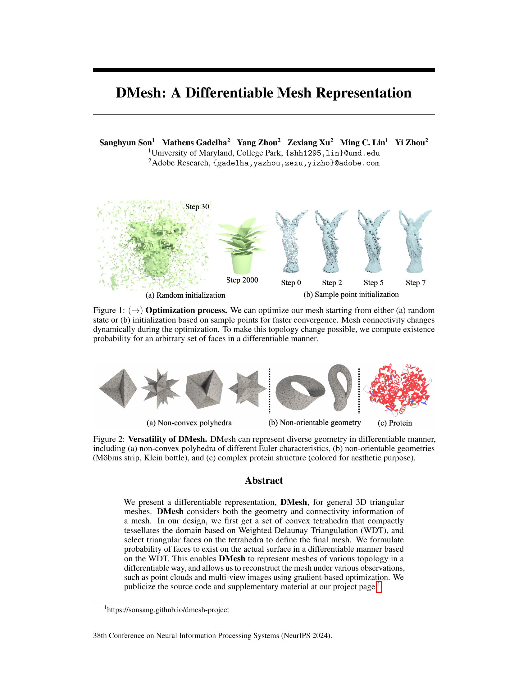
This figure shows the optimization process of DMesh. The left panel (a) demonstrates optimization starting from a random initialization of points, gradually forming a coherent mesh over iterations (steps 30 and 2000 shown). The right panel (b) shows optimization starting from an initialization based on sample points, leading to faster convergence to a refined mesh. The sequence of steps (0, 2, 5, 7) illustrates the dynamic changes in mesh connectivity during the optimization process, enabled by the differentiable computation of face existence probabilities.

This table presents the results of reconstructing three 3D mesh models (Bunny, Dragon, and Buddha) using the DMesh method. The results are evaluated using two metrics: * RE (Recovery Ratio): Percentage of faces in the ground truth mesh that were correctly recovered in the DMesh reconstruction. * FP (False Positive Ratio): Percentage of faces in the DMesh reconstruction that did not exist in the ground truth mesh. The table shows very high recovery ratios (above 99%) and relatively low false positive rates for all three models, indicating the effectiveness of the DMesh method in reconstructing meshes.
In-depth insights#
Diff Mesh Rep#
A differentiable mesh representation, often abbreviated as “Diff Mesh Rep,” is a significant advancement in 3D computer graphics and related fields. It allows for the seamless integration of mesh-based models into machine learning pipelines. Traditionally, meshes have been difficult to use directly within differentiable systems due to their discrete nature (connectivity of vertices and faces). A Diff Mesh Rep cleverly addresses this challenge by representing both the geometry and topology of a mesh in a manner that can be manipulated using gradient-based optimization techniques. This often involves probabilistic approaches to handle topological changes (e.g., merging or splitting faces) in a differentiable way. The key advantage is that this enables optimization algorithms to directly modify the shape and structure of meshes. This approach opens doors for applications in shape reconstruction, mesh generation, animation, and other areas that benefit from smooth, continuous representations. However, challenges remain, including computational cost and dealing with non-manifold meshes (meshes with inconsistencies in connectivity). Further research focuses on improving efficiency and robustness while retaining the benefits of differentiability.
WDT Optim.#
The heading ‘WDT Optim.’ likely refers to the optimization of Weighted Delaunay Triangulation (WDT) within a differentiable mesh representation. This is a crucial component because WDT provides a robust and efficient way to create a tessellation of the 3D space, forming a foundation upon which the differentiable mesh is built. Efficient WDT optimization is key because it directly impacts the overall computational cost of the system. A computationally expensive WDT algorithm can significantly slow down the optimization process, making it challenging to handle high-resolution meshes. The authors likely explore methods to make WDT differentiable, a necessary step for gradient-based optimization of the mesh. Differentiable WDT allows for the mesh’s topology to change dynamically during optimization, handling non-convex and non-orientable geometries. The optimization strategy likely involves minimizing a loss function that considers both the geometry (vertex positions) and connectivity (probability of faces existing) of the mesh. This might incorporate regularizations to maintain desirable properties like mesh quality or simplification, improving computational performance and result quality. The success of the overall method hinges on this WDT optimization; an inefficient or inaccurate method would directly affect the accuracy and speed of mesh reconstruction from point clouds or multi-view images.
Reconstr. Loss#
The heading ‘Reconstr. Loss’, short for reconstruction loss, in a research paper about 3D mesh reconstruction, signifies the core methodology used to evaluate how well a generated mesh aligns with the ground truth data. It quantifies the difference between a model’s output and the reference data, which can be a point cloud, a set of multi-view images, or a previously existing mesh. The effectiveness of various mesh optimization techniques is directly measured by the magnitude of the reconstruction loss. A lower reconstruction loss indicates a more accurate and faithful reconstruction, highlighting the efficacy of the proposed methods and algorithms. This loss function plays a critical role in guiding the iterative optimization process, driving improvements in the mesh’s geometry and connectivity to better match the target shape. The precise formulation of the reconstruction loss, therefore, is highly dependent on the type of input data used and may involve various metrics such as Chamfer distance or photometric error, combined to create a holistic measure of reconstruction quality. Ultimately, the reconstruction loss acts as the primary objective function that the model strives to minimize, offering a quantitative means for evaluating the performance of a novel 3D mesh reconstruction system.
Future Works#
The “Future Work” section of a research paper on differentiable mesh representations offers exciting avenues for improvement and expansion. Addressing the computational cost, especially for high-resolution meshes, is paramount. Exploring alternative approaches that lessen reliance on the computationally expensive Weighted Delaunay Triangulation would significantly enhance scalability. Tackling the non-manifoldness issue is another key area; strategies to ensure manifold meshes, perhaps by integrating techniques from signed distance fields or other implicit surface representations, could improve mesh quality and downstream applications. Further research could focus on expanding the applications of differentiable meshes. This involves considering handling more complex geometries, such as those with intricate details or non-orientable surfaces, integrating additional features (texture, color, etc.), and applying the mesh representation to various applications like generative models for 3D shapes and 3D reconstruction from real-world imagery.
Mesh Limits#
The heading ‘Mesh Limits’ in a research paper likely discusses the boundaries and constraints inherent in representing shapes using meshes. This could involve exploring limitations in mesh resolution, such as the trade-off between detail and computational cost. Another aspect might be topological limitations, examining difficulties in representing shapes with complex or non-orientable topologies (like Möbius strips) accurately using meshes. Numerical stability is a key area, where meshing algorithms may produce inaccurate or unstable results in certain situations. The discussion could further analyze the efficiency of mesh processing operations, such as smoothing, simplification, or Boolean operations. Finally, ‘Mesh Limits’ might discuss limitations related to data representation, exploring how input data (like point clouds) influences the quality and effectiveness of the resulting mesh. In essence, this section would provide a critical analysis of the capabilities and inherent weaknesses of using meshes for shape modeling within the context of the research.
More visual insights#
More on figures

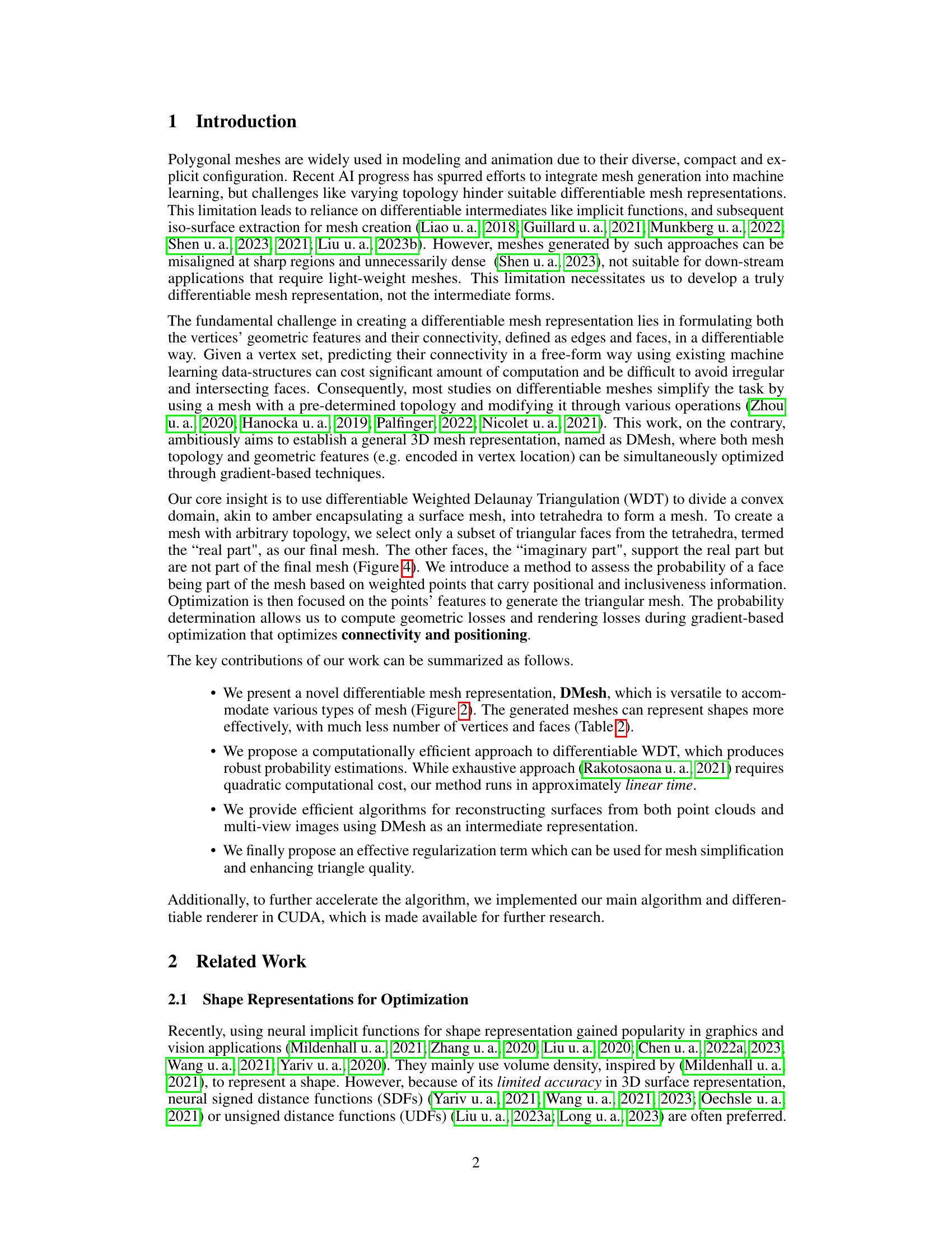
This figure demonstrates the versatility of the DMesh representation by showcasing its ability to represent various 3D shapes, including non-convex polyhedra with different topological properties, non-orientable surfaces like the Möbius strip and Klein bottle, and a complex protein structure. The image visually confirms that DMesh can handle a wide range of geometric complexities and topological features.

This figure illustrates the overall framework for optimizing a mesh based on given observations. It breaks down the process into four stages: (a) Point representation: Each point has a 5D feature vector (position, weight, real value). (b) Face probability: The system identifies potentially existing faces and calculates their probability. (c) Loss computation: Reconstruction loss is calculated based on the input (mesh, point cloud, or images). (d) Regularization: Additional regularization terms are added to improve mesh quality.

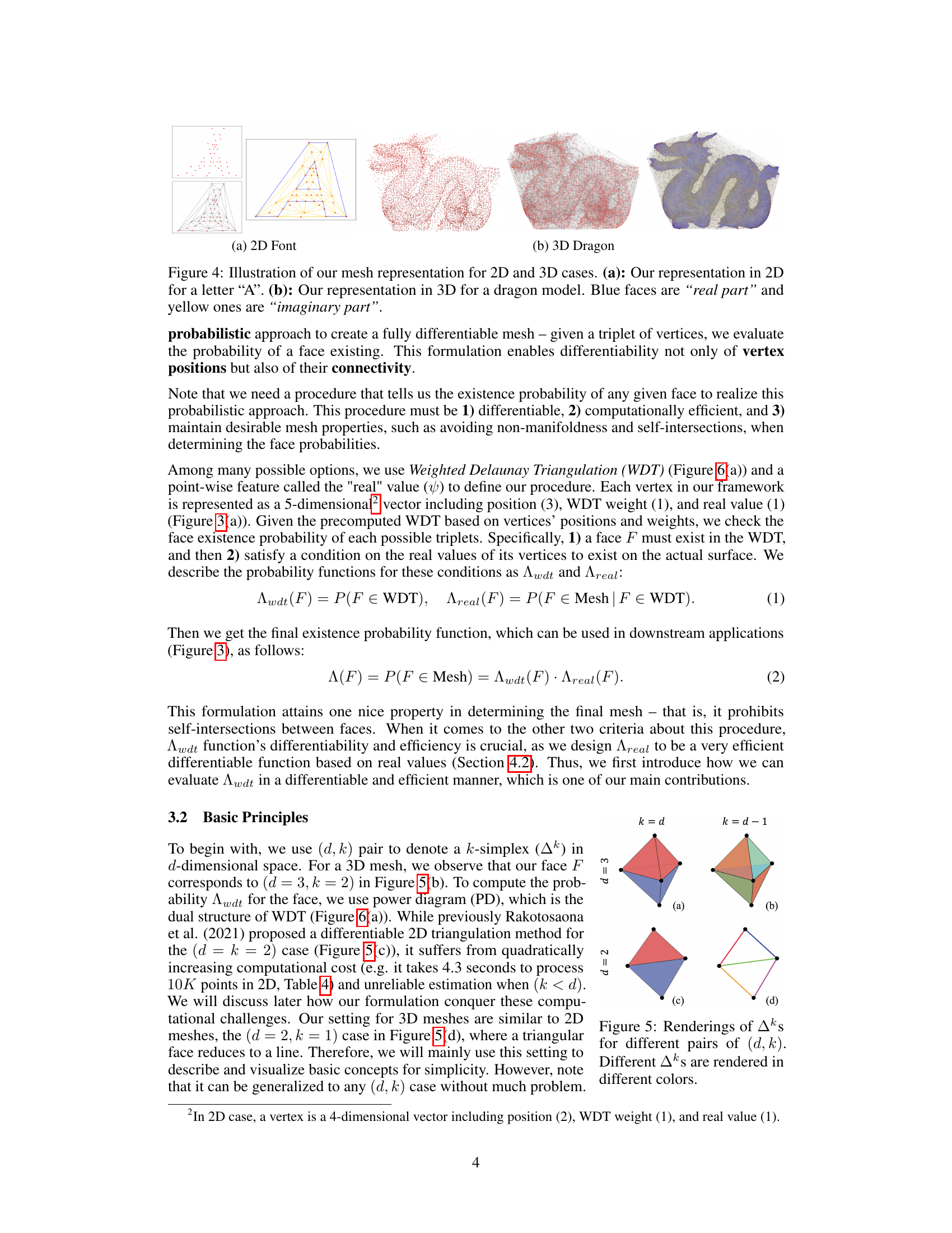
This figure shows two examples of how the DMesh representation works. In 2D, a letter ‘A’ is constructed from a set of points and their connections. The blue faces represent faces that belong to the final mesh, while the yellow ones are auxiliary faces that aid in constructing the mesh but are not part of it. In 3D, a dragon model is shown, where again, the blue faces represent the final mesh, and the yellow ones are auxiliary faces. The figure illustrates how the DMesh approach represents complex shapes probabilistically, handling both geometric and topological details of the mesh.
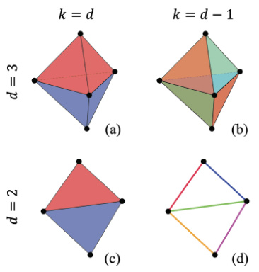
This figure illustrates the concept of k-simplex (Δk) in d-dimensional space. It shows different renderings of Akd, which represents the existence probability of a k-simplex in a d-dimensional space. The figure visually represents how the probability calculation changes depending on the dimensionality (d) and the number of vertices in the simplex (k). Different colors are used to distinguish different Akd values.

This figure illustrates the core concepts behind computing the existence probability of a 1-simplex (a line segment between two weighted points) within a Weighted Delaunay Triangulation (WDT). Panel (a) shows the WDT and its dual, the Power Diagram (PD). Panel (b) highlights the power cell (Cp1) of a point p1, illustrating its relationship with the 1-simplex (∆¹) and its dual line (D△1). Panels (c) and (d) introduce the concept of a ‘reduced’ power cell (Rp1|△1), which excludes a specific point from the WDT, allowing for a differentiable measure of simplex existence based on the distance between the dual line and the reduced power cell.

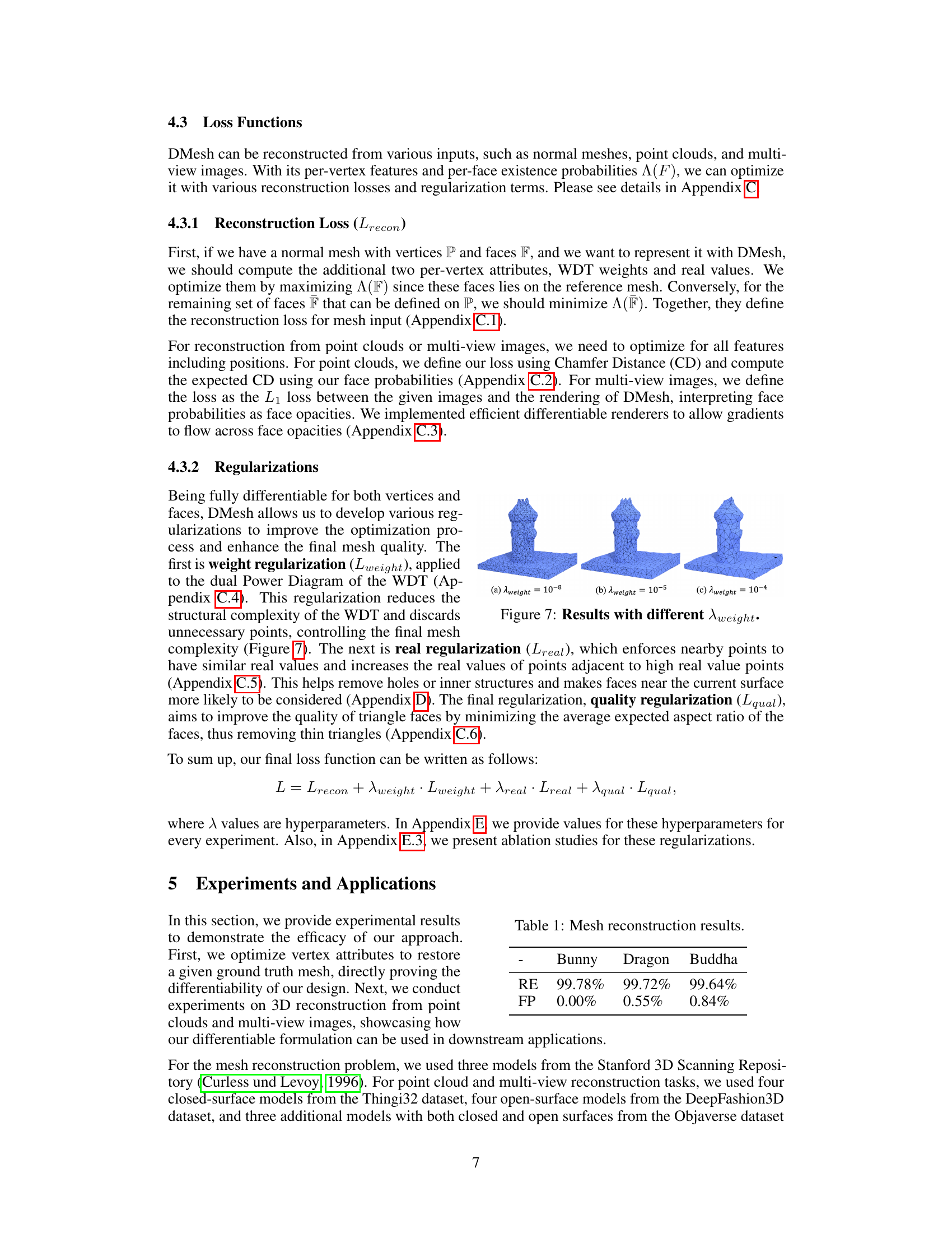
This figure shows the results of the weight regularization with different hyperparameters (λweight). The images illustrate how varying λweight influences the complexity of the mesh. A smaller λweight (10⁻⁸) results in a more complex mesh, while larger values (10⁻⁵ and 10⁻⁴) produce simpler meshes. This demonstrates the effect of the weight regularization on mesh simplification.
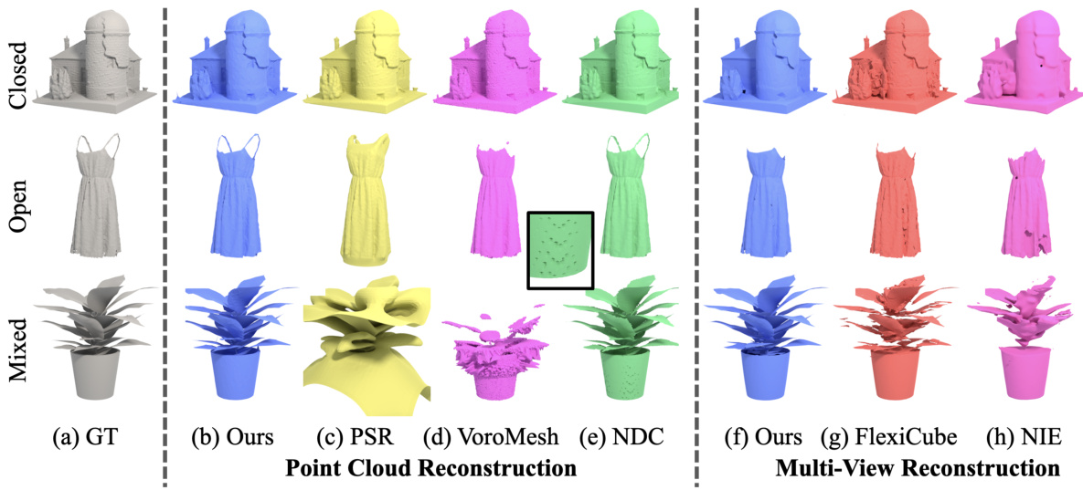
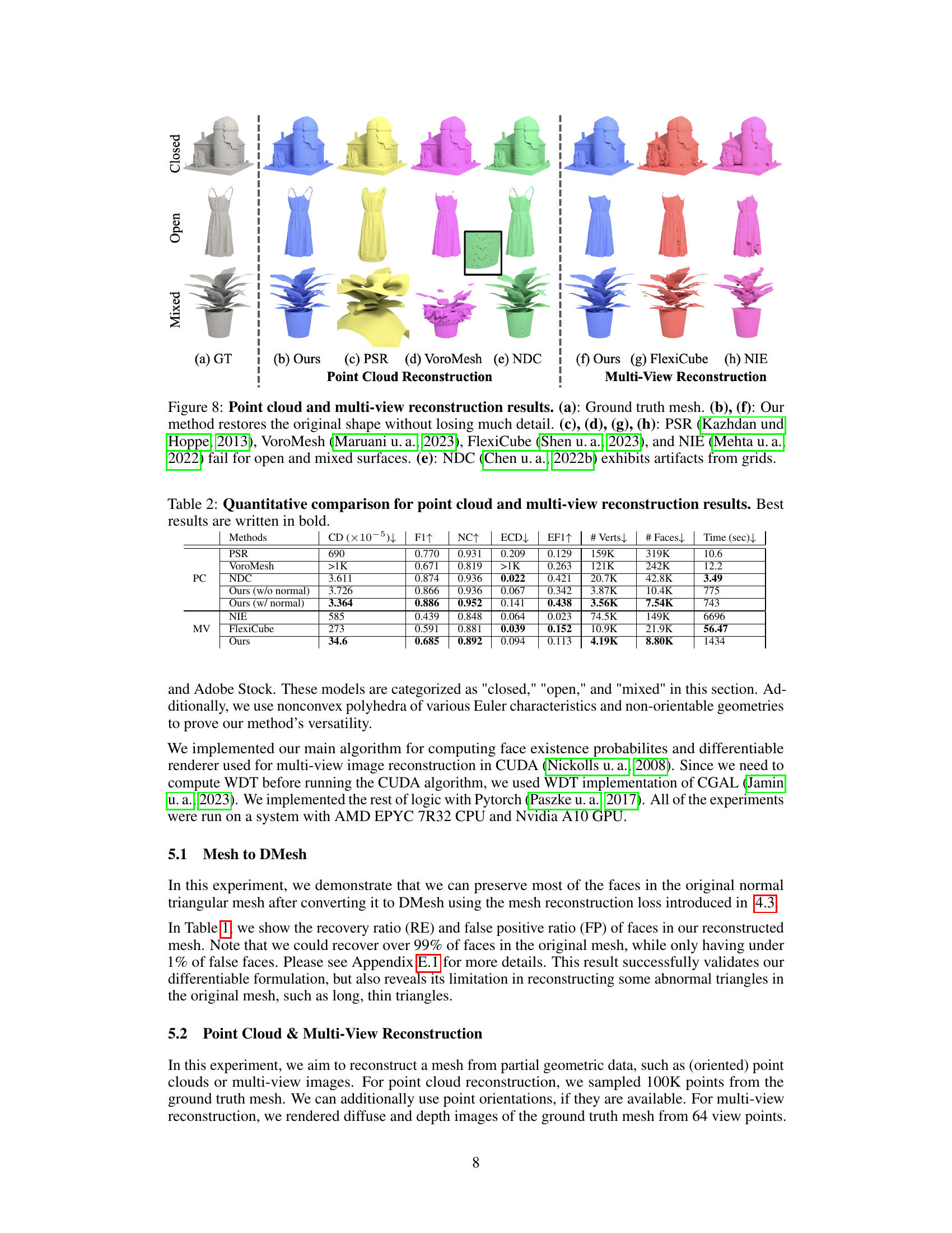
This figure compares the results of point cloud and multi-view reconstruction using the proposed DMesh method with several other state-of-the-art methods. It demonstrates the ability of DMesh to accurately reconstruct meshes, particularly those with open or mixed surfaces, where other methods struggle. The ground truth meshes are shown for comparison, highlighting DMesh’s superior performance in detail preservation and handling of surface complexity.

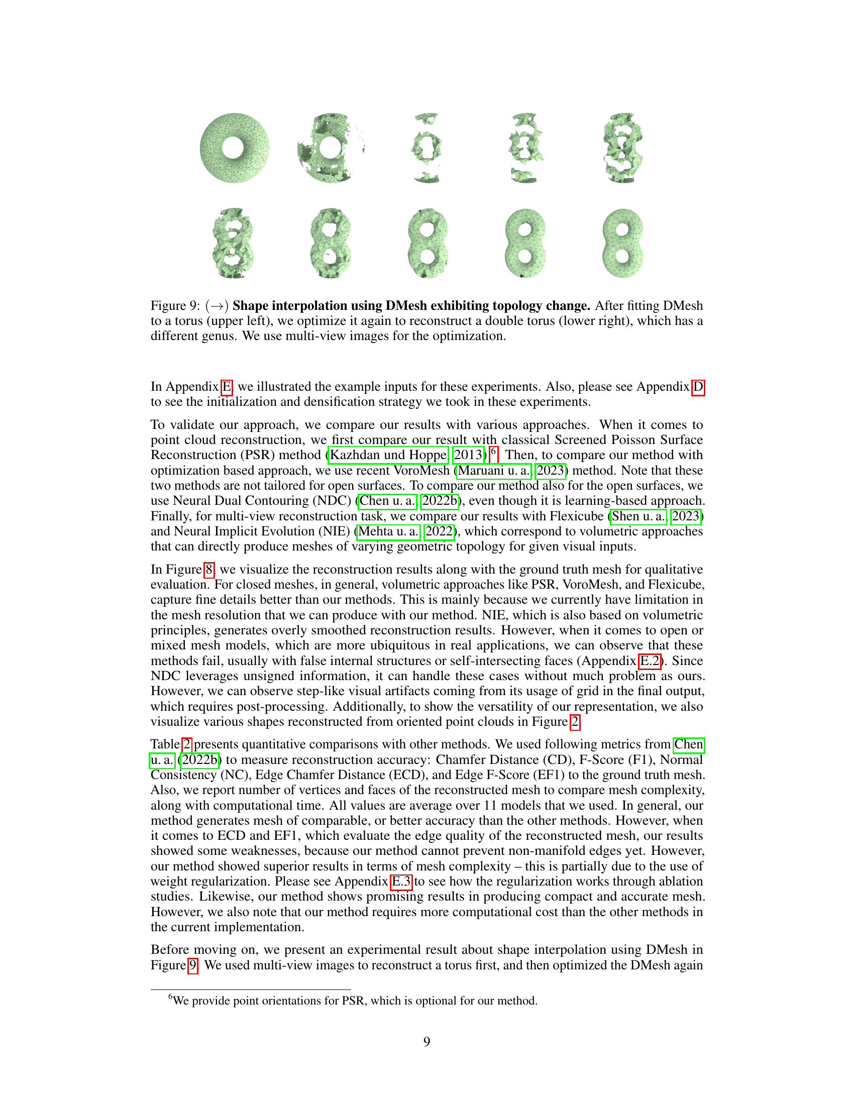
This figure shows the process of shape interpolation using DMesh. Starting with a torus, the model is optimized using multi-view images to gradually transform it into a double torus, demonstrating DMesh’s ability to handle topology changes during optimization.

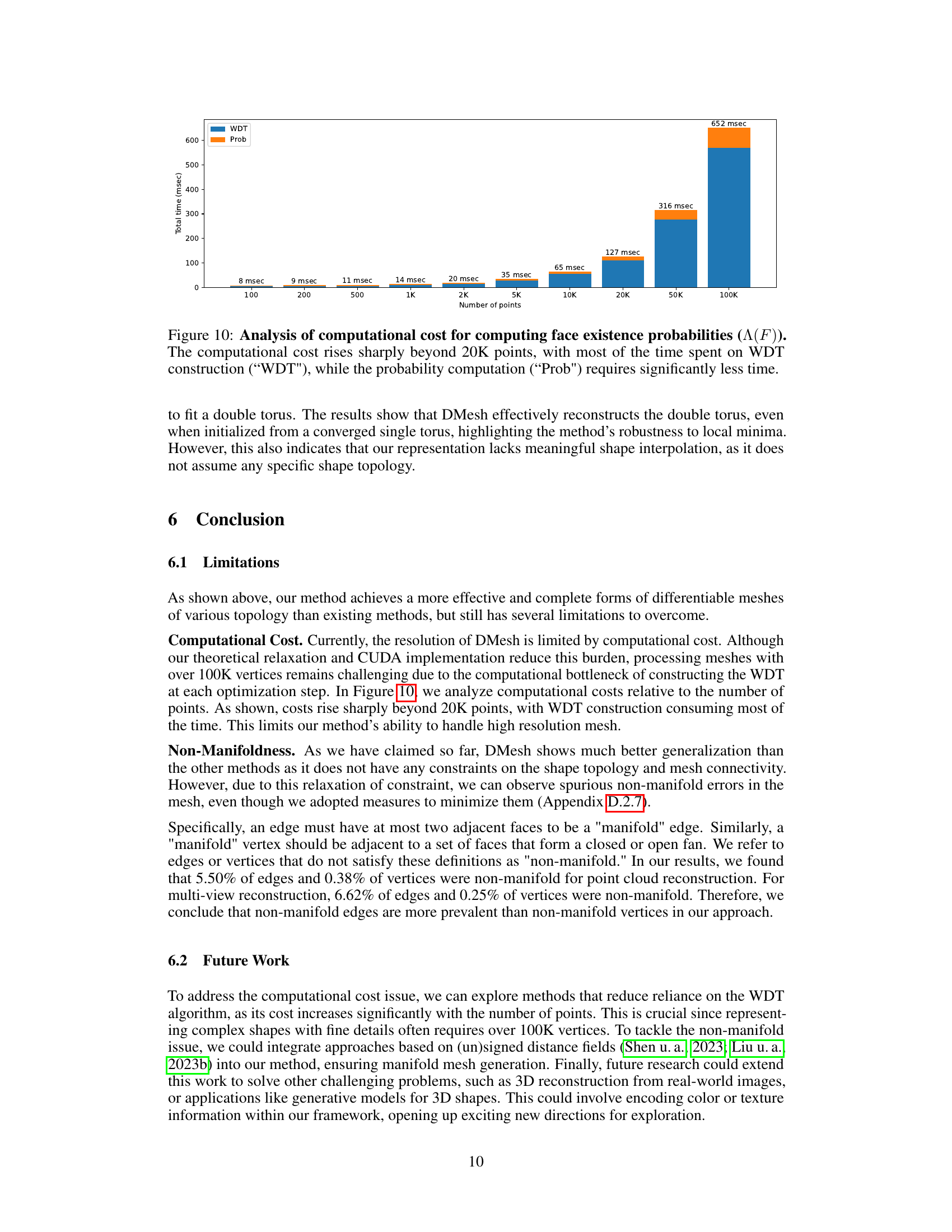
This bar chart visualizes the computational cost breakdown for calculating face existence probabilities in the DMesh method, categorized into WDT construction and probability computation. It reveals a significant increase in computation time beyond 20,000 points, primarily driven by the WDT construction. The probability computation remains relatively efficient.
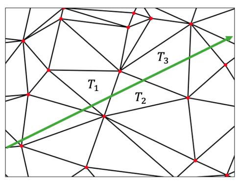
This figure illustrates the tessellation structure used in the second differentiable renderer (FB). A ray tracing through the scene intersects a sequence of triangles (tetrahedra in 3D). The structure ensures that when a ray enters a triangle through one edge, it proceeds to the next adjacent triangle only through a different edge of the current triangle. This allows efficient depth sorting without explicit depth testing, reducing computational cost and memory usage. The green line in the figure represents a sample ray tracing across the triangles.

This figure shows the results of rendering using two different renderers, FA and FB. Renderer FA is a partially differentiable tile-based approach, while FB, based on Laine et al. (2020), is used to supplement FA because FA lacks visibility-related gradients needed for accurate results. The comparison highlights the strengths and weaknesses of each rendering method for producing diffuse and depth images.
This figure shows how the authors initialize DMesh using sample points from a ground truth mesh. The left image (a) illustrates the uniform sampling of 10,000 points from the ground truth mesh. The right image (b) displays two different point sets: the sampled points (red) and the Voronoi vertices (blue). The initial mesh generated from these points is also shown (right image, right side), which has holes. The figure demonstrates one of the methods to initialize the parameters of the DMesh.
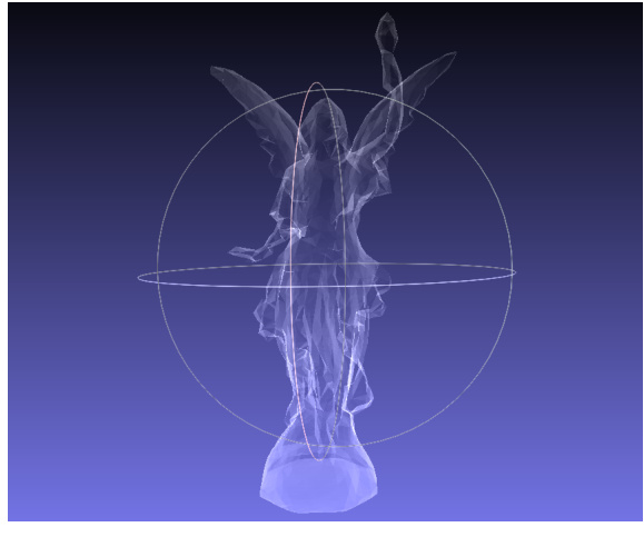
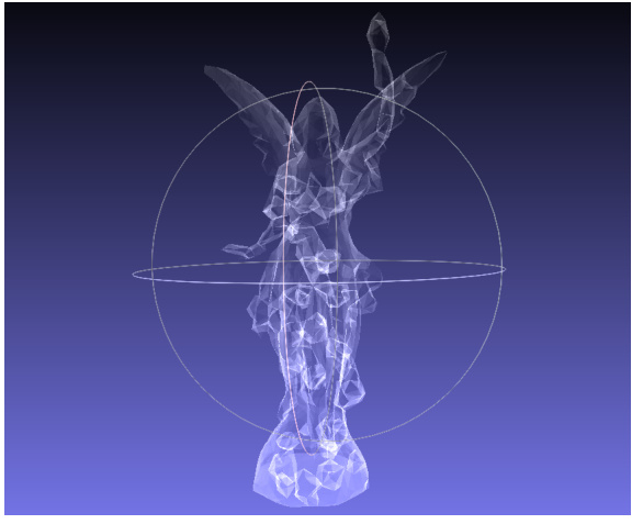
This figure shows the results of multi-view reconstruction using DMesh. It highlights a two-phase optimization process. The first phase uses a fast, but less precise, renderer leading to some incorrect inner faces. The second phase employs a more accurate renderer to refine the mesh and remove these artifacts. The x-ray rendering in MeshLab reveals the inner structure.

This figure shows the intermediate steps of converting a bunny model into DMesh representation. (a) shows the ground truth bunny mesh. (b) shows the initialization step where the initial DMesh is a convex hull around the bunny. (c) shows the point insertion step where additional points are added to problematic regions of the mesh. (d) shows the result after 5000 optimization steps, demonstrating that the model has largely recovered the connectivity of the original mesh.
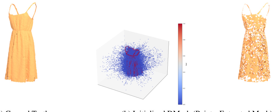
This figure shows the initialization of DMesh using sample points from a ground truth mesh. Subfigure (a) illustrates the uniform sampling of 10,000 points from the ground truth mesh. Subfigure (b) presents two visualizations: one showing the sampled points in red and the Voronoi vertices in blue, and another depicting the initial, incomplete mesh generated from these points, highlighting its many holes. This initialization technique leverages the proximity of Voronoi vertices to the medial axis of the shape.
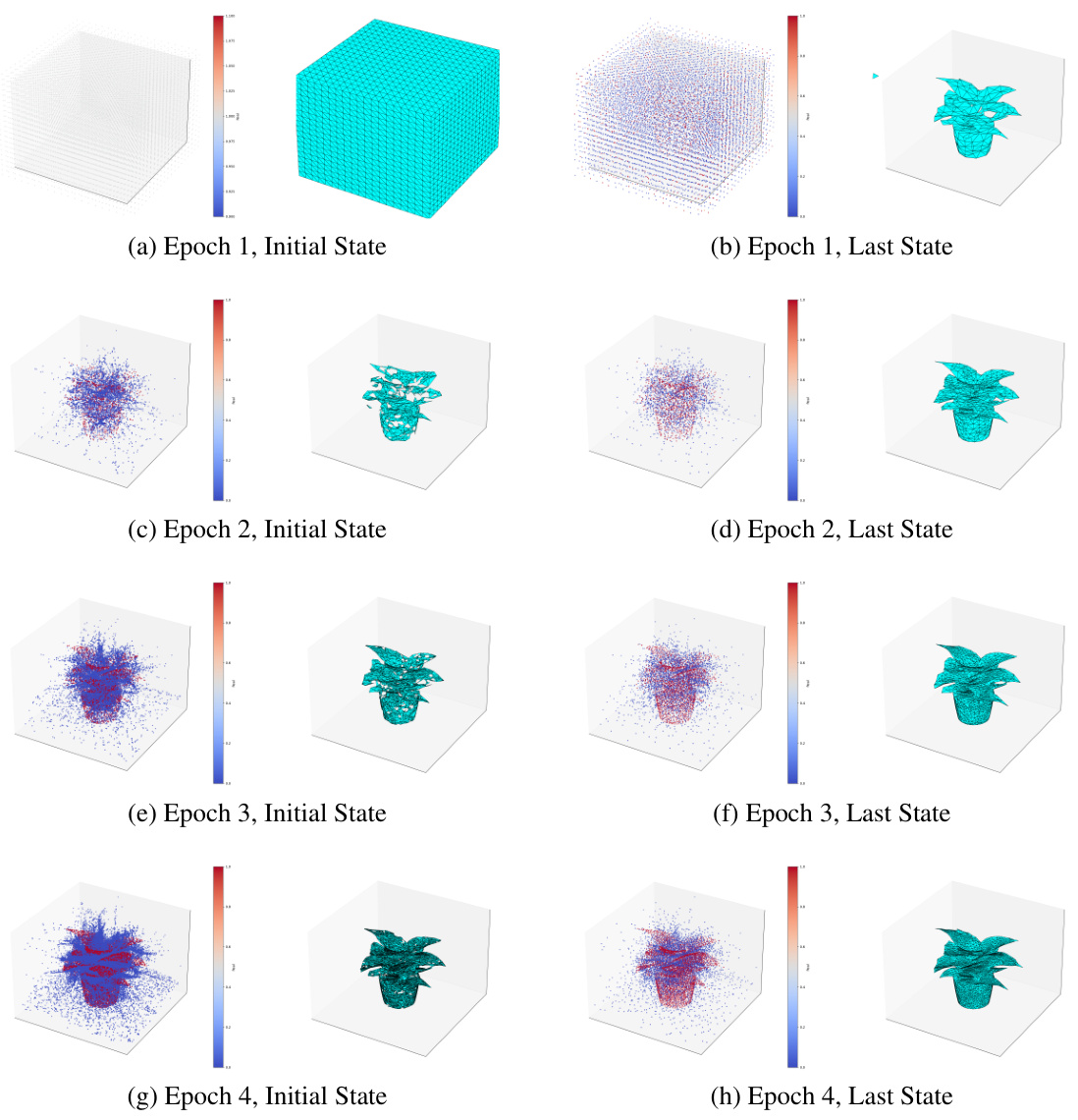
This figure shows the optimization process of DMesh for multi-view reconstruction of a plant model over four epochs. Each epoch starts with an initial state (left column) and ends with a last state (right column). The left images display the initial point distribution with colors representing the real values of the points, while the right images show the resulting 3D mesh after optimization. The first epoch begins without pre-existing sample points, and subsequent epochs utilize sampled points from the previous epoch’s mesh for initialization, refining the mesh iteratively.
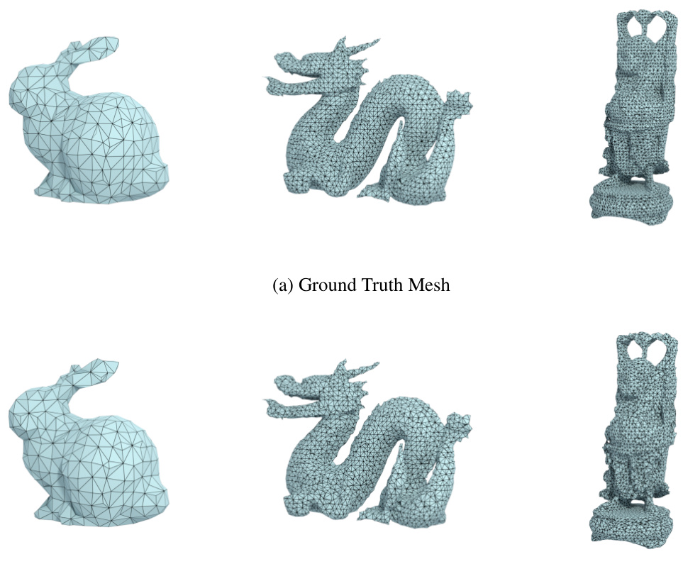
This figure shows the results of converting three different meshes (Bunny, Dragon, and Buddha) into DMesh. The left column shows the original meshes, while the right column shows the corresponding DMesh reconstructions. The results demonstrate the method’s ability to accurately preserve the connectivity of the original mesh, with only minor differences in appearance due to small positional adjustments during optimization.

This figure compares the reconstruction results of a closed surface model from the Thingi32 dataset using three different methods: the ground truth mesh, the Flexicube method, and the DMesh method proposed in the paper. The Flexicube method produces a mesh with some internal structures, while the DMesh method produces a cleaner mesh without these internal structures. This comparison highlights one of the advantages of the DMesh method, which is its ability to produce cleaner meshes by removing internal structures during post-processing.
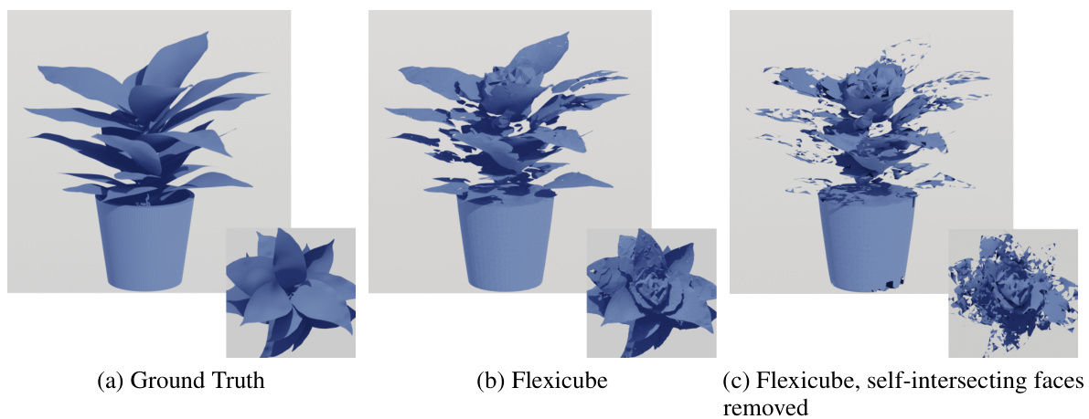
This figure compares the reconstruction results of the Plant model using the proposed DMesh method and the Flexicube method. It highlights that Flexicube tends to produce redundant and self-intersecting faces, particularly for open surfaces like the leaves of the plant. The DMesh method avoids this issue.
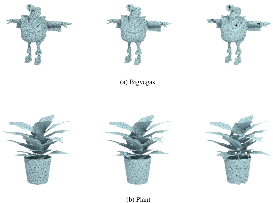
This figure shows the optimization process of DMesh for multi-view reconstruction of a plant model across four epochs. Each epoch starts with an initialization, either from scratch or using samples from the previous epoch’s results. The left side displays the initial point attributes color-coded by real values, while the right shows the mesh extracted at each epoch’s end. The process demonstrates how the mesh progressively refines over epochs, incorporating more points, and more accurately representing the target object.

This figure shows the optimization process of DMesh for multi-view reconstruction of a plant model. Each row displays the initial and final states of the model in each epoch. The left column shows the point attributes color-coded by their real values, while the right column shows the extracted mesh. The first epoch starts without sample points, and subsequent epochs utilize sample points from the previous epoch’s mesh for initialization. This illustrates the iterative refinement process of the DMesh optimization.

This figure shows the results of point cloud and multi-view reconstruction experiments on four different open-surface models. For each model, it displays (from left to right): the ground truth mesh, the sampled point cloud used as input, the reconstructed mesh from the point cloud, the diffuse rendering of the reconstructed mesh, and finally, the reconstructed mesh from multi-view images. The figure demonstrates the capability of DMesh to reconstruct open surfaces from both point cloud and multi-view data.
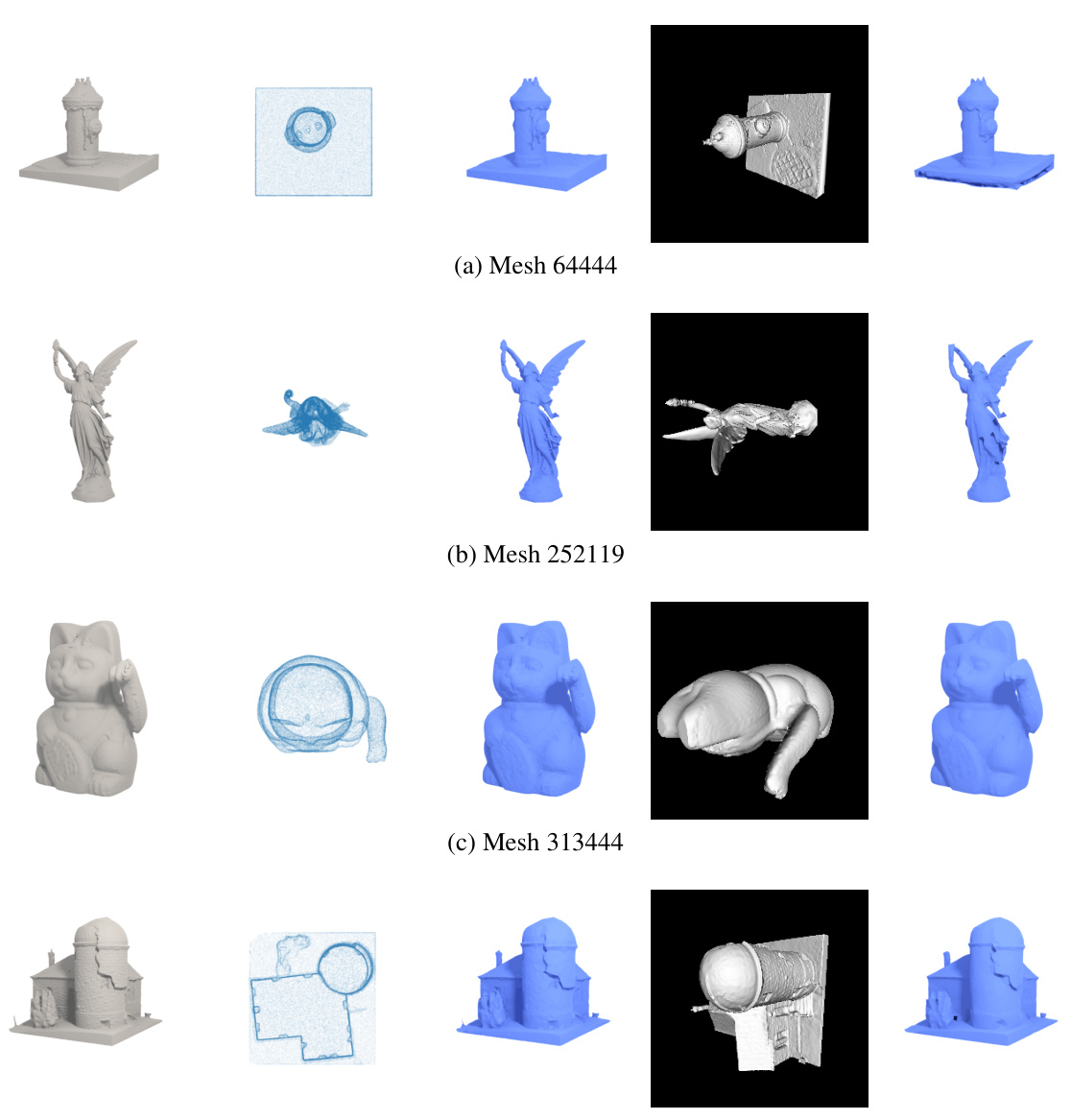
This figure shows the results of applying the DMesh method to reconstruct 3D models from point cloud and multi-view image data. The figure presents four different closed-surface models. For each model, it displays: (a) the ground truth mesh, (b) a sample point cloud used as input for reconstruction, (c) the mesh reconstructed from the point cloud, (d) a diffuse rendering of the reconstructed mesh, and (e) the mesh reconstructed from multi-view images. The results demonstrate the method’s ability to accurately reconstruct 3D shapes from different input data types.

This figure compares the results of point cloud and multi-view reconstruction using the proposed DMesh method with other state-of-the-art methods. The results show that DMesh effectively reconstructs the original shapes without losing much detail, unlike other methods that often fail to reconstruct open and mixed surfaces or exhibit artifacts. The ground truth mesh is displayed, followed by the results from DMesh, PSR, VoroMesh, NDC, FlexiCube, and NIE.
More on tables

This table presents a quantitative comparison of different methods for point cloud and multi-view reconstruction. It compares the methods using several metrics: Chamfer Distance (CD), F1-score (F1), Normal Consistency (NC), Edge Chamfer Distance (ECD), and Edge F1-score (EF1). It also shows the number of vertices and faces in the generated meshes, and the computation time. The best results for each metric are highlighted in bold. The metrics are used to evaluate the accuracy and efficiency of each reconstruction method.

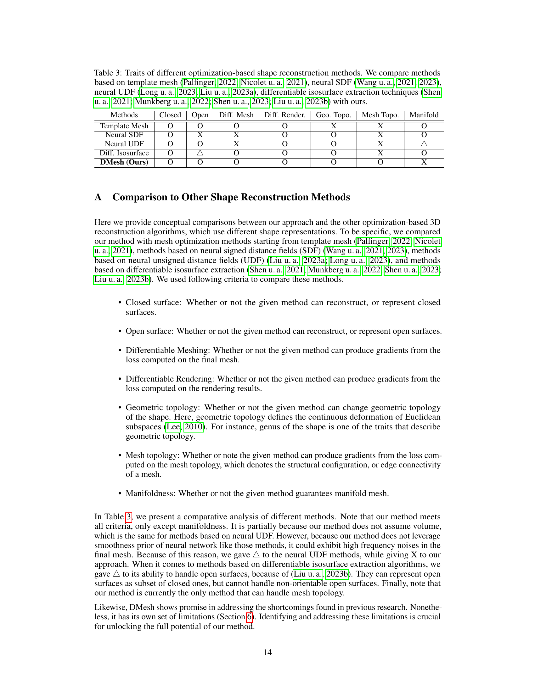
This table compares several mesh reconstruction methods based on different techniques, including template mesh, neural signed distance fields (SDF), neural unsigned distance fields (UDF), and differentiable isosurface extraction. The comparison focuses on the methods’ ability to handle closed and open surfaces, whether they offer differentiable meshing and rendering, and their capacity for geometric and mesh topology changes, as well as the manifold property of their output meshes. The table highlights the unique capabilities and limitations of each approach, including DMesh (the authors’ method).

This table compares various mesh reconstruction methods based on different criteria. The methods are categorized by their approach to mesh representation (template mesh, neural SDF, neural UDF, differentiable isosurface extraction) and compared against the proposed DMesh method. The criteria used for comparison include whether the method supports closed or open surfaces, differentiable meshing and rendering processes, geometric and mesh topology changes, and the resulting mesh’s manifoldness. Each method is evaluated based on the presence (O) or absence (X) of these traits, with Δ indicating a partial or conditional presence of a trait.

This table presents the ablation study of the weight regularization. For different lambda_weight values (10^-6, 10^-5, 10^-4), the Chamfer Distance (CD) and the number of faces in the reconstructed mesh are compared. It shows a trade-off between mesh complexity (number of faces) and reconstruction accuracy (CD). Lower lambda_weight values lead to lower CD but higher number of faces, while higher lambda_weight values show higher CD but fewer faces.

This table compares several optimization-based 3D shape reconstruction methods based on different shape representations. It compares methods using template meshes, neural signed distance fields (SDF), neural unsigned distance fields (UDF), and differentiable isosurface extraction. The comparison is made across several criteria, including whether the methods handle closed and open surfaces, support differentiable meshing and rendering, and allow changes in geometric and mesh topology. It also indicates if the resulting mesh is guaranteed to be manifold.
Full paper#
