TL;DR#
Current weather forecasting models, primarily data-driven, struggle with fine-grained temporal resolution due to their “black-box” nature and reliance on limited training data. This inability to extrapolate to shorter time intervals hinders the accuracy of nowcasting and precise short-term predictions, which are crucial for many applications. The limited temporal resolution in datasets prevents these models from providing accurate predictions at finer time scales, leading to significant challenges in various sectors such as emergency response and urban planning.
To overcome these limitations, the researchers introduce WeatherGFT, a novel physics-AI hybrid model. This model integrates physical laws (PDEs) to simulate fine-grained temporal evolution, coupled with neural networks for bias correction and a lead-time-aware training strategy. This approach enables WeatherGFT to produce accurate 30-minute forecasts even when trained solely on hourly data. Extensive experimental results across different lead times show WeatherGFT outperforms state-of-the-art methods, highlighting the effectiveness of the physics-AI hybrid approach in enhancing weather forecasting capabilities.
Key Takeaways#
Why does it matter?#
This paper is important because it addresses a critical limitation of current ML-based weather forecasting models, which struggle to generalize to finer temporal scales than those present in their training data. By proposing a novel physics-AI hybrid model, WeatherGFT, this research opens new avenues for accurate and high-resolution weather forecasting across multiple time scales, thereby improving situational awareness and enabling better preparedness for extreme weather events. Its findings have implications for various applications, including disaster management, urban planning, and resource allocation.
Visual Insights#

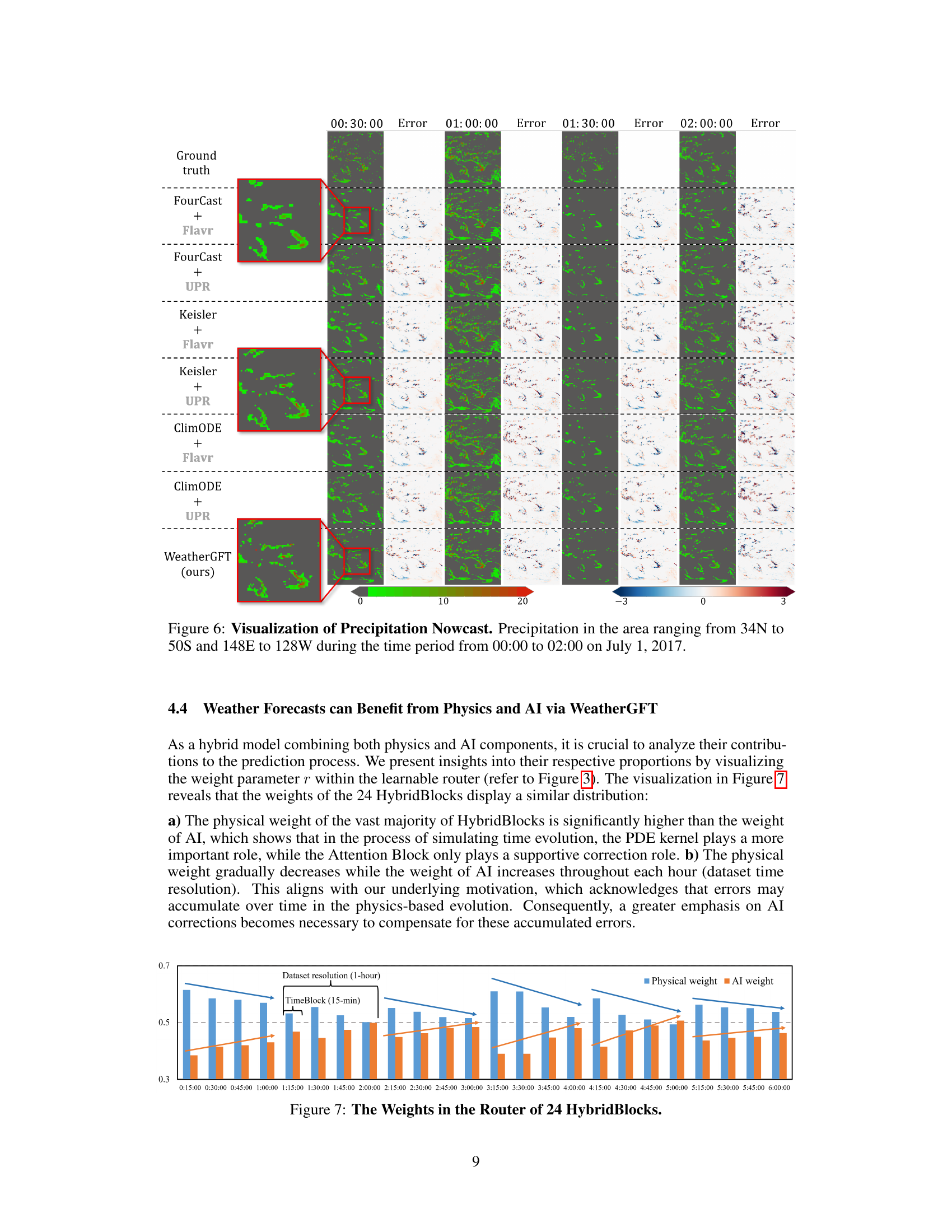
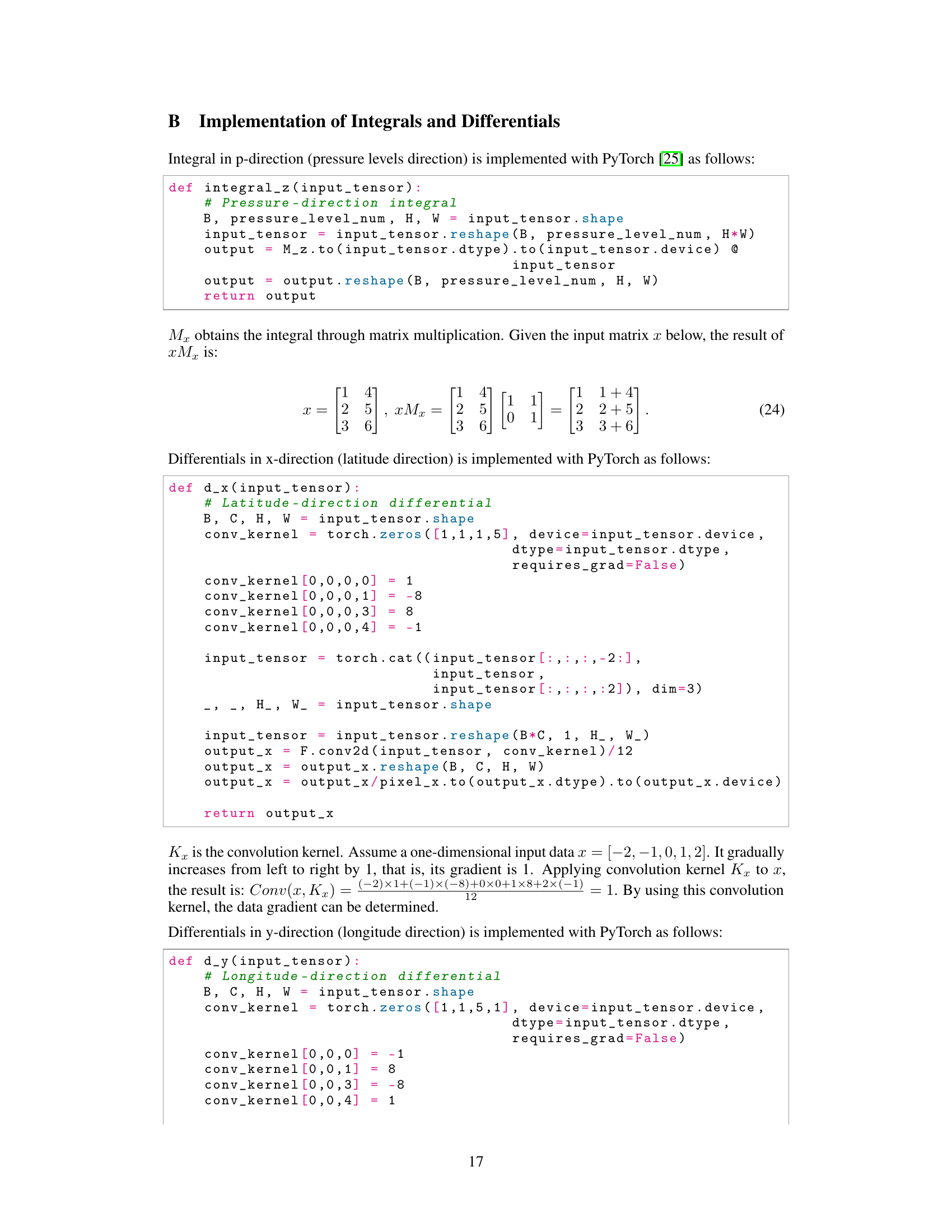
🔼 This figure shows the learnable router weights in the HybridBlock of the WeatherGFT model at different forecast lead times. The weights represent the proportion of the output from the physical (PDE) and AI (neural network) branches. Initially, both branches are weighted equally (0.5:0.5). As the lead time increases, the weight of the physics branch decreases, indicating error accumulation in the PDE simulations. Conversely, the weight of the AI branch increases, showing that the AI component plays a more significant role in correcting for the errors at longer lead times. This demonstrates the adaptive nature of the hybrid model, where physics drives the primary evolution and AI performs adaptive bias correction.
read the caption
Figure 1: Learnable router weight. The role of physics and AI at different lead times: major evolution and adaptive correction (details in Sec. 4.4).

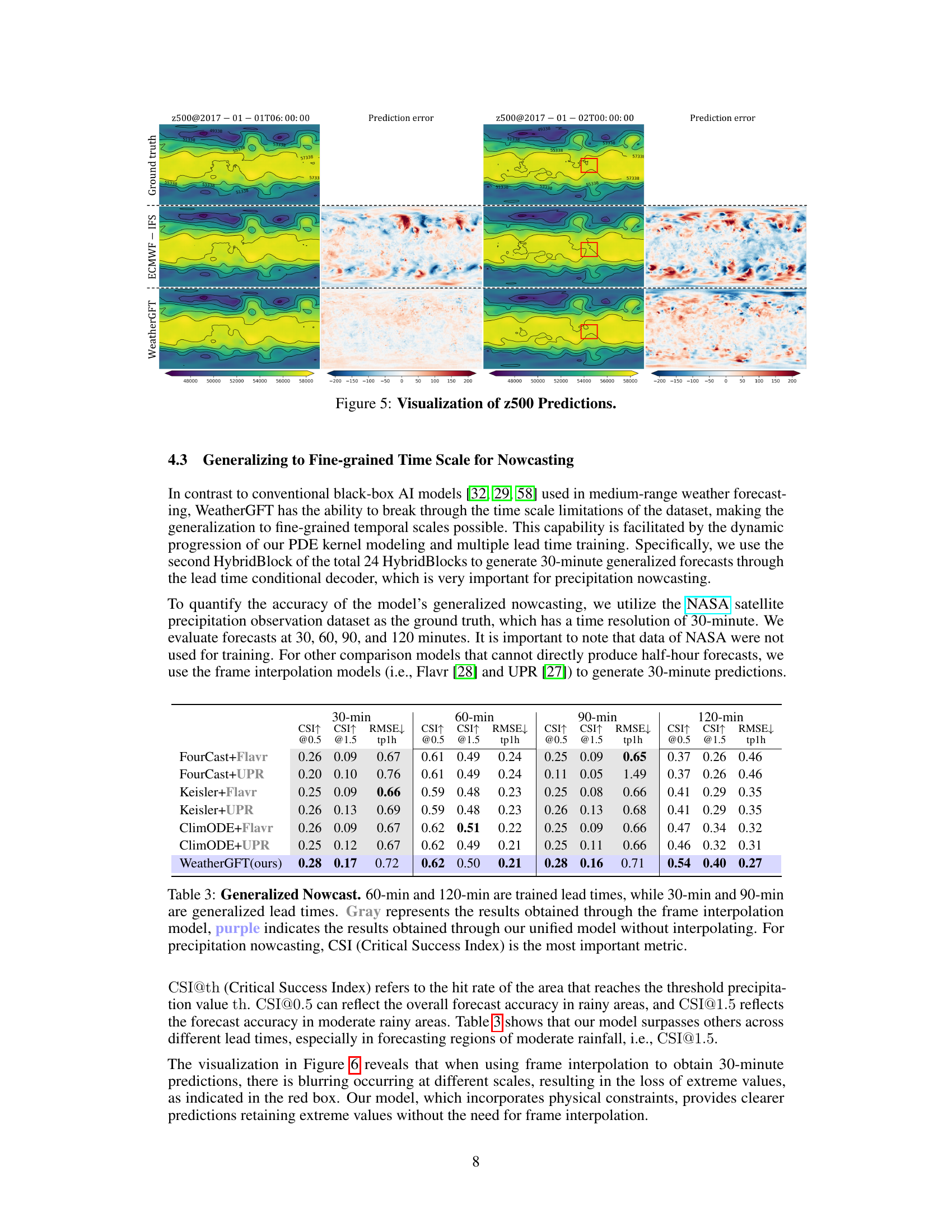
🔼 This table compares the performance of WeatherGFT and other models on a nowcasting task, specifically predicting precipitation at various lead times (30, 60, 90, and 120 minutes). It highlights WeatherGFT’s ability to generate 30-minute forecasts, which are not present in the training data, outperforming models that rely on frame interpolation to produce those finer-grained forecasts. The Critical Success Index (CSI) at thresholds of 0.5 and 1.5 are used to evaluate forecast accuracy.
read the caption
Table 3: Generalized Nowcast. 60-min and 120-min are trained lead times, while 30-min and 90-min are generalized lead times. Gray represents the results obtained through the frame interpolation model, purple indicates the results obtained through our unified model without interpolating. For precipitation nowcasting, CSI (Critical Success Index) is the most important metric.
In-depth insights#
Physics-AI Synergy#
The concept of ‘Physics-AI Synergy’ in weather forecasting represents a powerful paradigm shift. Instead of solely relying on black-box AI models, which excel at pattern recognition but lack understanding of underlying physical processes, a hybrid approach integrates physical models (PDEs) with AI. The physical models provide a strong foundation for simulating weather evolution, especially at fine-grained temporal scales where data scarcity hinders purely data-driven methods. AI components then serve to refine the physical model’s predictions, correcting biases and improving accuracy. This synergy is crucial as it leverages the strengths of both approaches: the explanatory power and physical consistency of physics and the adaptability and bias correction capabilities of AI. The learnable router mechanism dynamically weights the contributions of both modules at different lead times, highlighting their complementary roles and enhancing model generalizability across various forecast horizons. This approach potentially leads to more accurate and reliable weather forecasts, particularly at finer temporal resolutions currently beyond the reach of conventional methods.
Fine-grained Forecasts#
The concept of “Fine-grained Forecasts” in weather prediction signifies a significant leap towards more precise and timely weather information. Traditional forecasting methods often operate on coarser temporal and spatial scales, resulting in less accurate predictions, especially for short-term events. The pursuit of fine-grained forecasts addresses this limitation by aiming for higher resolution in both time and space. This requires advancements in data acquisition, model design, and computational power. Data-driven AI models, coupled with physical simulations, are key components in achieving this goal. The challenge lies in balancing the accuracy of AI’s learning capabilities with the fidelity of physical laws governing weather phenomena. Successful fine-grained forecasts depend on effective integration of these two approaches to generate more reliable, detailed, and ultimately beneficial predictions for various applications, from emergency management to agricultural planning.
PDE-Kernel Fusion#
The concept of “PDE-Kernel Fusion” suggests a powerful approach in physics-informed machine learning. It likely involves combining the strengths of partial differential equation (PDE) models, which capture the underlying physical dynamics of a system, and machine learning models, which can learn complex patterns from data. The fusion likely aims to leverage PDEs to provide strong inductive biases, guiding the learning process and improving generalization performance, especially in scenarios with limited data. This fusion might take the form of incorporating PDE kernels directly into the neural network architecture or using PDEs to pre-process or post-process the data fed to the machine learning model. Successful PDE-kernel fusion is likely to lead to hybrid models that balance the accuracy and interpretability of PDEs with the flexibility and pattern-recognition capabilities of machine learning. Such a method could allow for accurate and detailed predictions even in situations where traditional PDE models are insufficient or data is scarce. A critical aspect would be the design of the fusion mechanism, ensuring that the PDE kernel effectively interacts with the machine learning component, preventing conflicts or hindering the learning process. The effectiveness would hinge on the chosen fusion architecture, the training strategy, and the overall system design, leading potentially to accurate, efficient, and physically consistent predictions.
Lead-Time Awareness#
Lead-time awareness in forecasting models is crucial for improving accuracy and generalization. A model with this awareness isn’t just predicting future states based on current conditions; it’s explicitly considering the time elapsed since the observation. This is particularly important for high-frequency forecasting, where subtle changes can dramatically affect short-term predictions. For example, a model lacking lead-time awareness might misjudge a rapidly intensifying storm because it doesn’t properly weigh the accelerating changes over time. Incorporating lead time can be done through various techniques, such as specialized architectures with time-aware layers or by designing loss functions that penalize errors differently across various forecast horizons. The benefit is twofold: enhanced short-term prediction accuracy, as the model dynamically adapts to rapidly evolving conditions, and better generalization to unseen lead times, reducing the overfitting to specific training horizons. The key is to find the optimal balance between learning the short-term evolution’s specifics and utilizing longer-term trends for accurate, adaptable forecasts.
Generalization Limits#
The heading ‘Generalization Limits’ in a research paper would explore the boundaries of a model’s ability to perform well on unseen data. A thoughtful analysis would delve into several aspects. First, it would examine the data distribution, questioning how closely the training data reflects the real-world scenarios the model will encounter. A mismatch could lead to poor generalization. Second, the study might investigate the model’s complexity. Overly complex models might overfit the training data, capturing noise and failing to generalize effectively, while overly simplistic models might underfit, missing crucial patterns. Third, it would address the representativeness of features. Does the model capture essential characteristics or only superficial aspects? Fourth, algorithmic biases need assessment; inherent biases in the algorithms themselves might hinder the model’s ability to fairly generalize. Finally, the discussion should address the temporal aspect of generalization. A model that works well for a specific time range may fail when applied to data outside this timeframe. Addressing these limitations requires careful consideration of dataset construction, model architecture, and bias mitigation techniques.
More visual insights#
More on figures
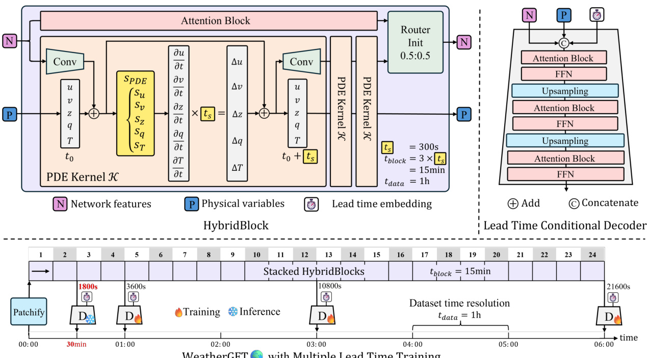
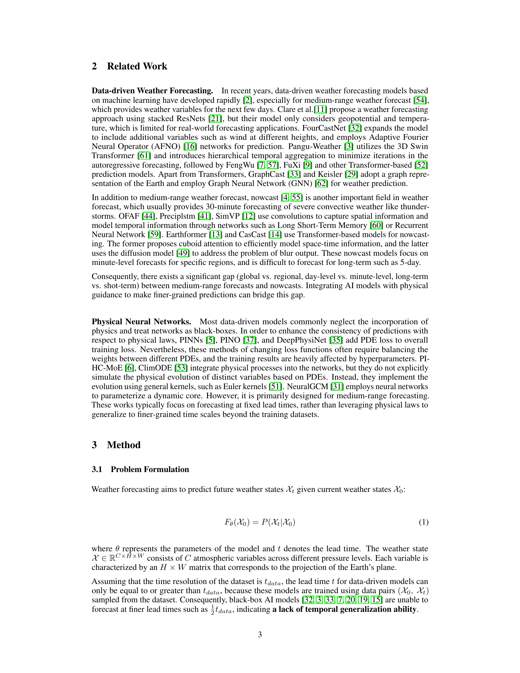
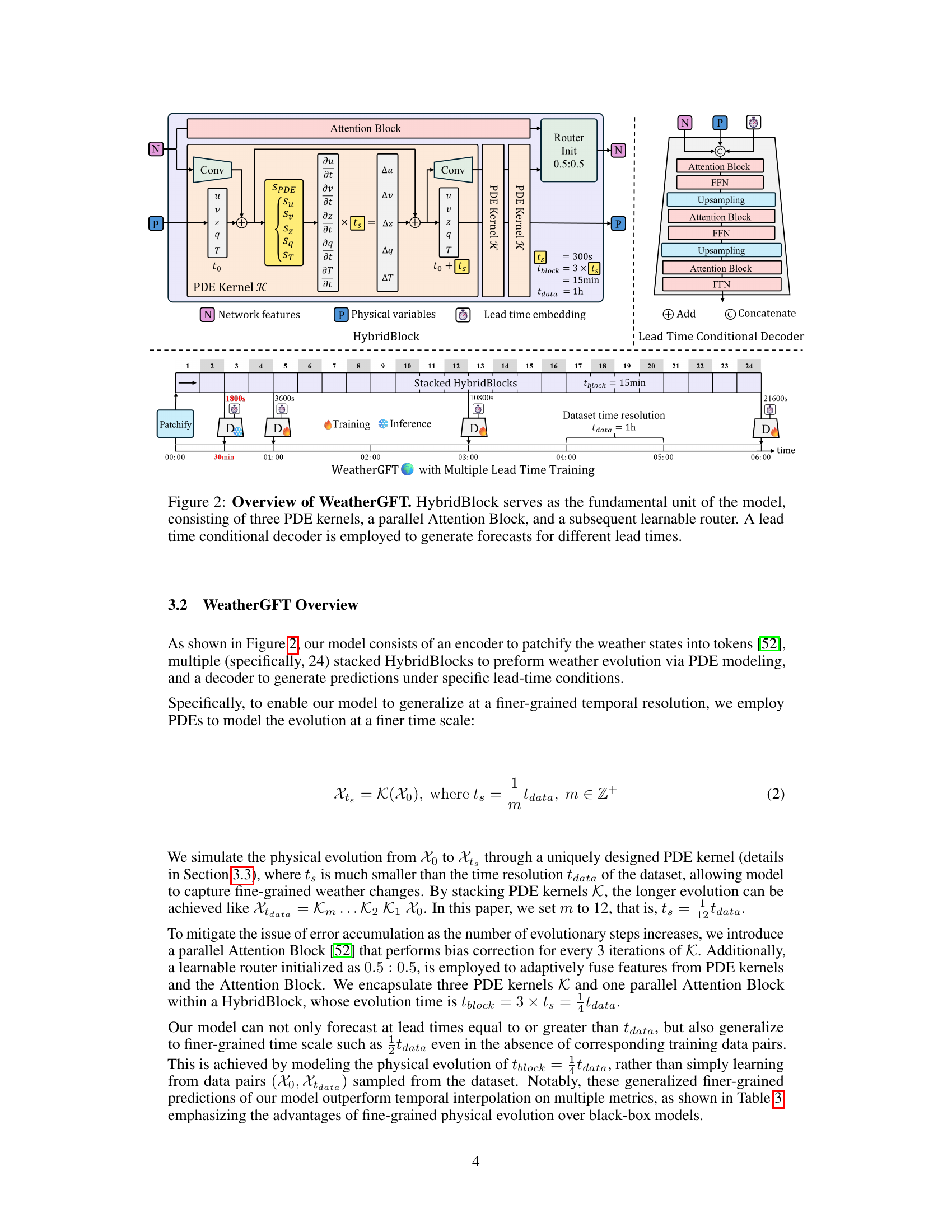
🔼 The figure provides a detailed overview of the WeatherGFT model architecture. It highlights the key components: the encoder for converting input weather data into tokens, the stacked HybridBlocks that form the core of the model, and the lead time conditional decoder that enables the model to predict forecasts at various lead times. Each HybridBlock contains a set of PDE (Partial Differential Equation) kernels for simulating physical evolution, a parallel Attention Block for bias correction, and a learnable router that adapts the fusion of physical and neural network outputs. This design allows the WeatherGFT model to generate fine-grained temporal resolution forecasts, exceeding the resolution of the training data.
read the caption
Figure 2: Overview of WeatherGFT. HybridBlock serves as the fundamental unit of the model, consisting of three PDE kernels, a parallel Attention Block, and a subsequent learnable router. A lead time conditional decoder is employed to generate forecasts for different lead times.

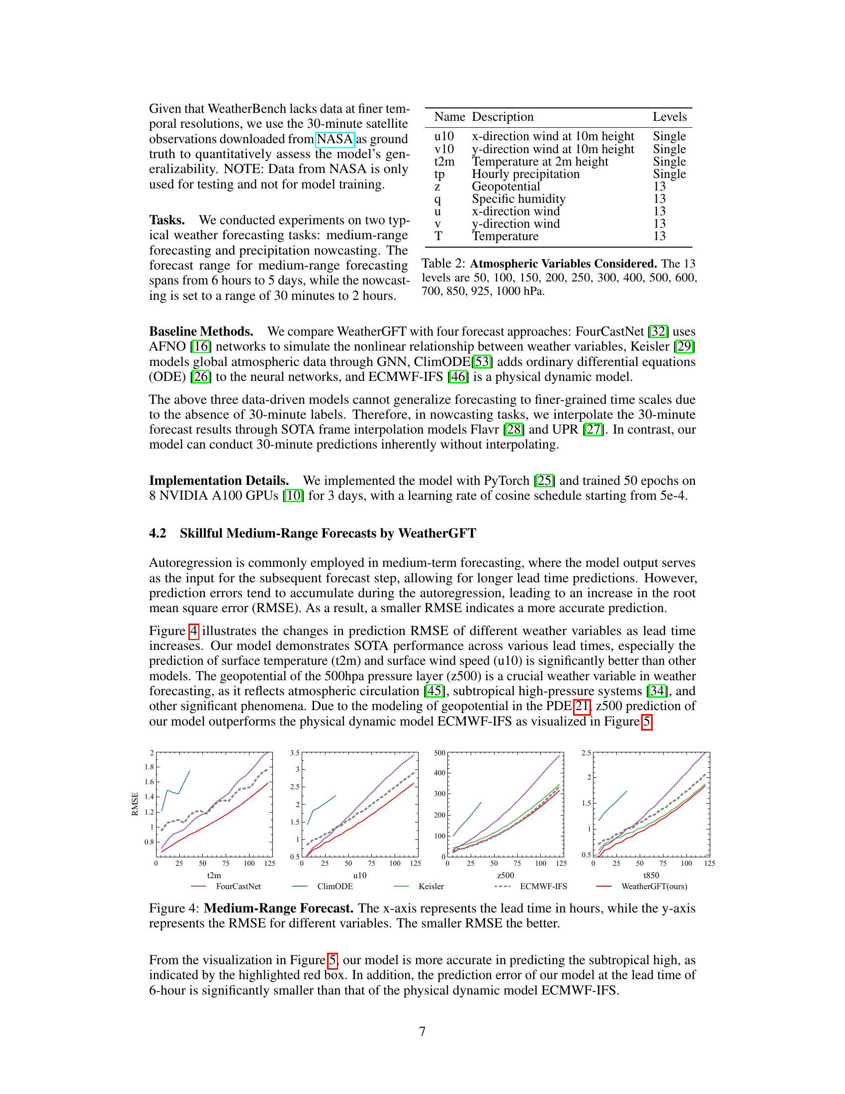
🔼 The figure shows the root mean square error (RMSE) for different weather variables (t2m, u10, z500, t850) predicted by different models (FourCastNet, ClimODE, Keisler, ECMWF-IFS, WeatherGFT) at various lead times (0-125 hours). A lower RMSE indicates better prediction accuracy. WeatherGFT consistently demonstrates superior performance across all variables and lead times.
read the caption
Figure 4: Medium-Range Forecast. The x-axis represents the lead time in hours, while the y-axis represents the RMSE for different variables. The smaller RMSE the better.

🔼 This figure visualizes the predictions of the geopotential at the 500hpa pressure layer (z500) using three different methods: WeatherGFT, ECMWF-IFS (a physical dynamic model), and ground truth. The visualization shows the predictions and their errors at two different time points (2017-01-01T06:00:00 and 2017-01-02T00:00:00). The red boxes highlight a region where WeatherGFT shows a smaller error compared to ECMWF-IFS, demonstrating improved accuracy in a specific region.
read the caption
Figure 5: Visualization of z500 Predictions.
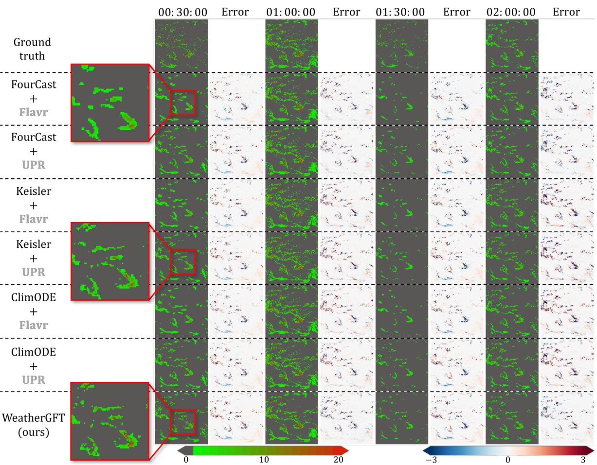
🔼 This figure visualizes the precipitation nowcast results from different models at various time points (00:30:00, 01:00:00, 01:30:00, and 02:00:00). It compares the ground truth precipitation data with predictions from FourCastNet combined with both Flavr and UPR interpolation methods, Keisler combined with both Flavr and UPR, ClimODE combined with both Flavr and UPR, and finally, the WeatherGFT model. The color scale represents the difference between predicted and ground truth precipitation, with green indicating accurate predictions and red/blue indicating underestimation and overestimation respectively. The red boxes highlight specific areas where the WeatherGFT model’s performance stands out.
read the caption
Figure 6: Visualization of Precipitation Nowcast. Precipitation in the area ranging from 34N to 50S and 148E to 128W during the time period from 00:00 to 02:00 on July 1, 2017.

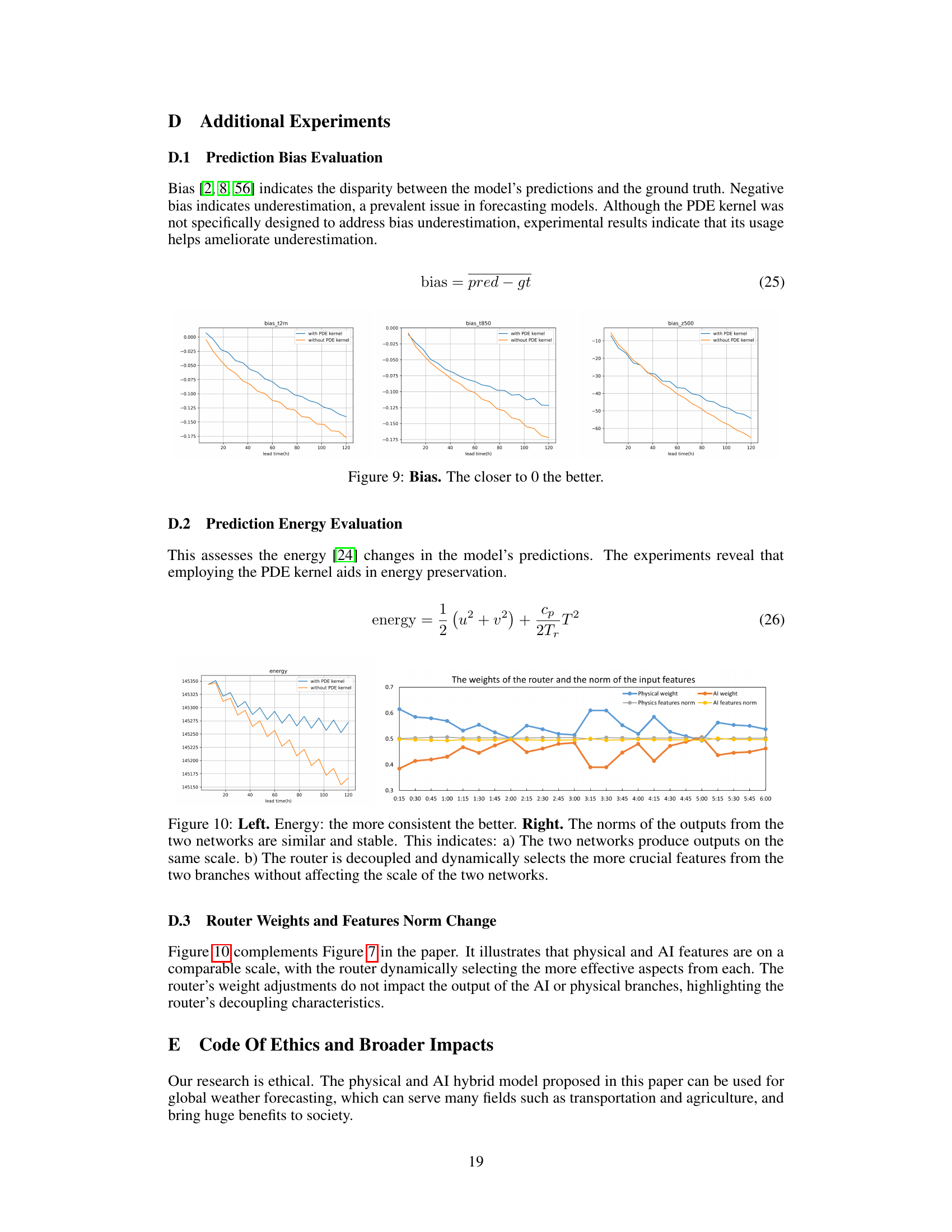
🔼 This figure visualizes the weights of the learnable router within each of the 24 HybridBlocks in the WeatherGFT model. The x-axis represents time, broken down into 15-minute intervals across a 6-hour period. The y-axis shows the weight assigned to either the physics or AI branch within each HybridBlock’s router. The figure demonstrates how the contribution of the physics-based branch gradually decreases over time, while the contribution of the AI-based correction branch increases to compensate for accumulating errors from the PDE kernel’s evolution.
read the caption
Figure 7: The Weights in the Router of 24 HybridBlocks.
🔼 The figure shows the Root Mean Square Error (RMSE) for different weather variables (t2m, u10, z500, t850) at different forecast lead times (0-125 hours). It compares the performance of WeatherGFT against three other models (FourCastNet, ClimODE, Keisler) and a physical dynamic model (ECMWF-IFS). Lower RMSE values indicate better forecast accuracy. The graph illustrates how the RMSE changes for each variable as the lead time increases, demonstrating the model’s skill in medium-range forecasting and its superiority to other methods for certain variables.
read the caption
Figure 4: Medium-Range Forecast. The x-axis represents the lead time in hours, while the y-axis represents the RMSE for different variables. The smaller RMSE the better.

🔼 This figure shows the bias (the difference between predictions and ground truth) for three variables (t2m, t850, z500) with and without the PDE kernel. Negative bias indicates underestimation. The results show that using the PDE kernel helps to reduce the bias, particularly for longer lead times.
read the caption
Figure 9: Bias. The closer to 0 the better.

🔼 The figure demonstrates the consistency of energy in the model’s prediction when using the PDE kernel. It also shows the normalization of the AI and physics outputs, which are similar, and that the router’s role in selecting features doesn’t affect the output scale.
read the caption
Figure 10: Left. Energy: the more consistent the better. Right. The norms of the outputs from the two networks are similar and stable. This indicates: a) The two networks produce outputs on the same scale. b) The router is decoupled and dynamically selects the more crucial features from the two branches without affecting the scale of the two networks.
More on tables

🔼 This table shows the datasets used in the paper. WeatherBench dataset is used for training and testing, with a time resolution of 1 hour. NASA dataset is only used for testing the 30-minute nowcasting task, providing ground truth precipitation data.
read the caption
Table 1: Datasets. NASA dataset only contains precipitation, which will be used as the ground truth for precipitation nowcast.

🔼 This table lists the atmospheric variables used in the WeatherGFT model, along with the number of pressure levels associated with each variable. The variables include surface-level measurements (wind speed and direction, temperature, and precipitation) and atmospheric profile data (geopotential, humidity, wind speed and direction, and temperature) across 13 pressure levels. The pressure levels are specified in hectopascals (hPa).
read the caption
Table 2: Atmospheric Variables Considered. The 13 levels are 50, 100, 150, 200, 250, 300, 400, 500, 600, 700, 850, 925, 1000 hPa.

🔼 This table presents the results of the generalized nowcasting experiments. It compares the performance of WeatherGFT against other models at various lead times (30, 60, 90, and 120 minutes). The Critical Success Index (CSI) at thresholds of 0.5 and 1.5, as well as the Root Mean Square Error (RMSE), are reported. Results are shown for models with and without frame interpolation, highlighting WeatherGFT’s ability to generalize to finer-grained timescales not present in its training data.
read the caption
Table 3: Generalized Nowcast. 60-min and 120-min are trained lead times, while 30-min and 90-min are generalized lead times. Gray represents the results obtained through the frame interpolation model, purple indicates the results obtained through our unified model without interpolating. For precipitation nowcasting, CSI (Critical Success Index) is the most important metric.

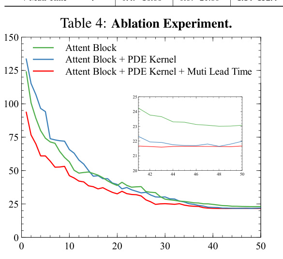
🔼 This table presents the results of ablation experiments conducted to evaluate the impact of different components of the WeatherGFT model on the 30-minute nowcast and medium-range forecasting tasks. The ‘Attent Block’ row represents the baseline model using only the attention block without PDE kernels or multi-lead time training. Subsequent rows progressively add the PDE kernel and multi-lead time training, showing the performance improvements of each addition. The RMSE (root mean square error) values for surface temperature (t2m) and 500 hPa geopotential (z500) are provided for lead times of 1 hour, 6 hours, and 3 days.
read the caption
Table 4: Ablation Experiment.
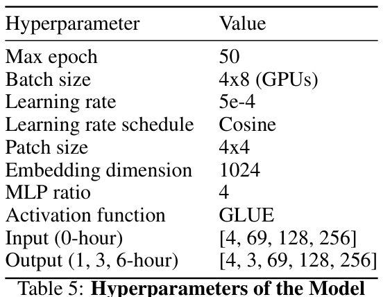
🔼 This table lists the hyperparameters used in the WeatherGFT model, including the maximum number of training epochs, batch size, learning rate and schedule, patch size, embedding dimension, MLP ratio, activation function, and input/output dimensions for different time horizons.
read the caption
Table 5: Hyperparameters of the Model

🔼 This table details the datasets used in the paper’s experiments. It lists the time period used for training, validation, and testing sets for both WeatherBench and NASA datasets. It also specifies the time resolution (1 hour for WeatherBench and 30 minutes for NASA) and the variables included in each dataset. Note that the NASA dataset only contains precipitation data (tp), while WeatherBench includes a broader range of meteorological variables.
read the caption
Table 6: Datasets Information
Full paper#


