TL;DR#
The hippocampus, vital for spatial and episodic memory, contains “place cells” whose activity reflects location. Current theories struggle to unify the spatial and episodic memory roles of the hippocampus. This paper investigates whether place cells can emerge from networks trained on temporally continuous sensory experiences.
The researchers modeled hippocampal region CA3 using a recurrent autoencoder, trained on data simulating an agent navigating virtual environments. Remarkably, the network developed place cell-like responses with key features like remapping, orthogonal representations in different environments, and robust emergence across various room shapes. This suggests that temporally continuous sensory experience is sufficient to generate spatial representations, potentially unifying spatial and episodic memory roles.
Key Takeaways#
Why does it matter?#
This paper is crucial because it offers a novel perspective on the emergence of place cells in the hippocampus, bridging the gap between spatial and episodic memory theories. Its findings have implications for understanding memory encoding and retrieval mechanisms, and it opens new avenues for research into virtual and abstract navigation. The testable predictions generated offer promising directions for future experimental studies.
Visual Insights#
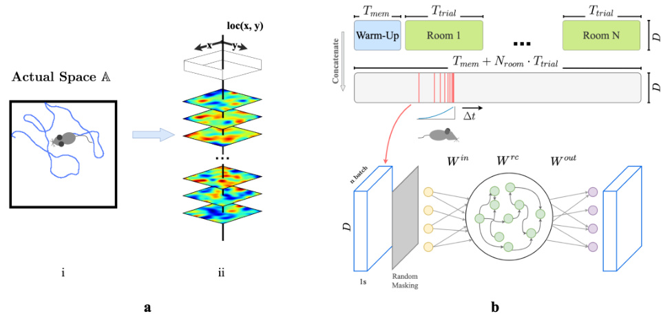
🔼 This figure shows the training schematic of the recurrent autoencoder (RAE) used in the study. Panel (a) illustrates how the agent’s trajectory in a 2D environment is converted into a sequence of sensory experience vectors. Panel (b) details the RAE architecture and training process, including random masking and noise addition to simulate realistic sensory experiences.
read the caption
Figure 1: a. (i) Example trajectory of an artificial agent in a 2D room in actual space A. (ii) Each room is defined by a unique set of weakly spatial modulated (WSM) signals representing location-dependent sensory cues. Within a room, a WSM rate map is defined by F = z *g(σ), F ∈ RW×H, where z is a 2D Gaussian random field. W and H are the dimensions of the room. A room is defined by its WSM set, i.e., R = [F1, F2, …, FD]T, R ∈ RD×W×H. b. Training schematic of our RAE. An artificial agent explores room(s) defined by a unique set of WSM signals, as depicted in panel a. Agents receive location-specific sensory experience vectors ex,y = R[:, x, y], where ex,y ∈ RD. The agent's trajectory within a trial is thereby converted into a sequence of experience vectors. At every training step, we randomly sample Nbatch segments of T, seconds from episodic memories within a Tw second window. These segments form a stack of memories used to train the RAE. Every EV in this stack is randomly masked to occlude between rmin to rmax% of the signal with added Gaussian noise €. The RAE is trained to reconstruct complete, noiseless experience vectors. The sampling window is shifted forward by At after each step until the end of the trial.

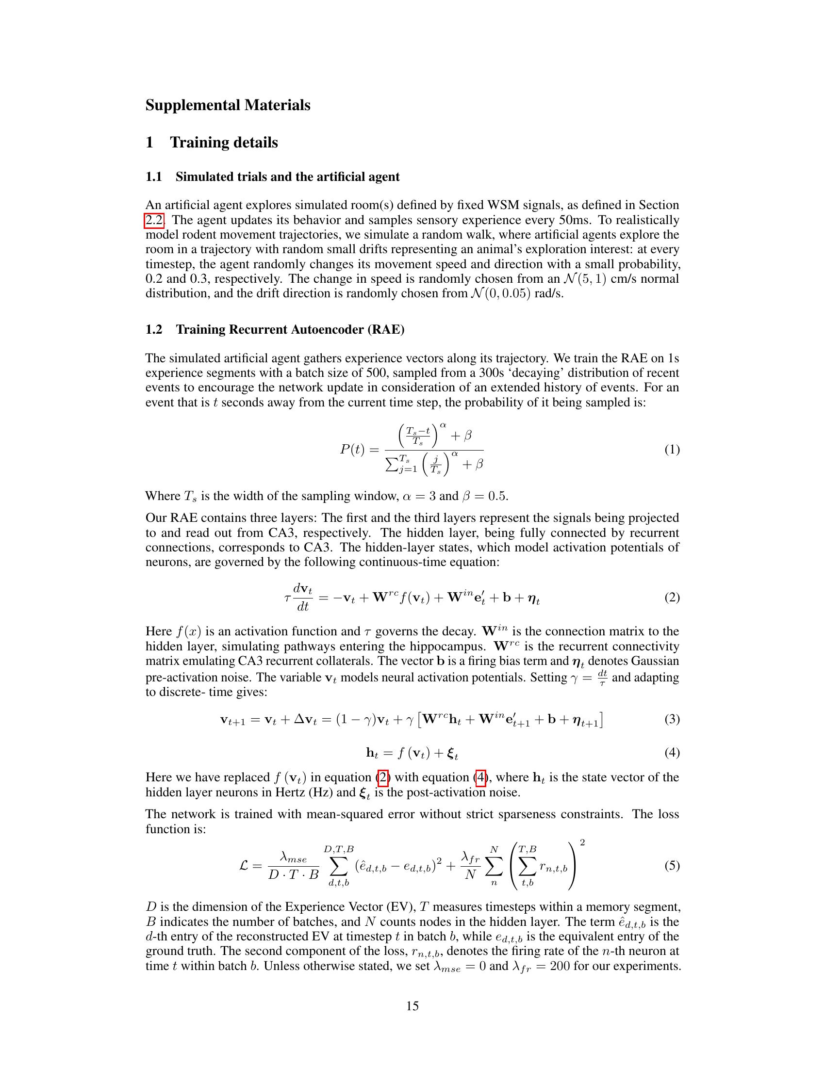
🔼 This table lists the hyperparameters used in the recurrent autoencoder model. It specifies the number of hidden layer nodes, the distribution of weights for the input, hidden, and output layers, the time resolution and time constant for the network dynamics, the decaying factor, the optimizer used, the learning rate, and the coefficients for the mean-squared error loss terms related to pattern completion and hidden layer firing rates.
read the caption
Table 1: Network parameters
In-depth insights#
Time Makes Space#
The intriguing title, “Time Makes Space,” encapsulates the core finding that continuous temporal experience, rather than explicit spatial information, is crucial for the emergence of place fields in neural networks. The research cleverly models the hippocampus as a recurrent autoencoder, learning to reconstruct temporally continuous sensory inputs from partial observations. This approach elegantly demonstrates that place cells, crucial for spatial navigation, spontaneously arise from the network’s attempt to accurately recall and reconstruct these temporally continuous experiences. The model successfully replicates key features of hippocampal place cells, including remapping and the formation of orthogonal representations in different environments. Furthermore, it suggests that the dimensionality of place fields is determined by the complexity of the temporally smooth sensory experiences, paving the way for testable predictions about how the environment shapes spatial representations in the brain. This work offers a compelling alternative perspective on the hippocampal spatial code, highlighting the significance of temporal continuity in shaping our perception of space.
Place Cell Emergence#
The emergence of place cells within the model is a significant finding, arising from the network’s attempt to reconstruct continuous sensory experiences. The key is the temporal continuity of the sensory data, mirroring an agent’s movement through space. This continuous input stream drives the network to create spatially localized firing patterns, rather than simply encoding individual snapshots of sensory information. The constraint on total network activity further encourages this spatial localization, leading to the emergence of place-like fields in the hidden layer. These fields show key properties of biological place cells, including remapping between different environments and the formation of orthogonal representations for distinct spaces. Importantly, the model reproduces these phenomena without explicitly encoding spatial information; the spatial representations arise naturally as a consequence of the temporally continuous, location-modulated sensory input. This suggests that the spatial properties of place cells may be an emergent property of networks encoding continuous experiences, rather than a result of hard-wired spatial maps. The model’s robustness across different room shapes and sizes further strengthens this conclusion.
Remapping & Reversion#
The concept of “Remapping & Reversion” in the context of spatial navigation and episodic memory is crucial. Remapping refers to the phenomenon where place cells, neurons that fire when an animal is in a specific location, adjust their firing patterns when the environment changes. This is adaptive, allowing the brain to create distinct spatial maps for different contexts. Reversion, conversely, highlights the remarkable ability of place cells to reactivate previous firing patterns when the animal returns to a familiar environment after exploring a novel one. This illustrates the hippocampus’s capacity for both flexibility in representing new spaces and stability in recalling past experiences. The interplay between remapping and reversion reveals the dynamic nature of spatial coding in the brain; a balance between adapting to new information while retaining access to previously learned representations. This is essential for efficient navigation and the formation of robust episodic memories, where context plays a pivotal role in retrieval.
Robust Place Fields#
The concept of “Robust Place Fields” in hippocampal research highlights the reliable and consistent firing patterns of place cells despite various environmental changes or internal factors. This robustness is crucial for the hippocampus’ role in spatial navigation and memory. Factors contributing to this robustness likely include the network’s recurrent connectivity and the integration of multiple sensory cues, allowing for pattern completion and separation even under noisy or incomplete sensory information. The ability of place cells to maintain stable firing fields across different contexts is essential, and the mechanisms underlying this stability remain a topic of active investigation. Further research will likely focus on understanding how the brain resolves conflicting spatial information and how plasticity in the hippocampus contributes to the adaptive remapping of place fields, enabling spatial navigation and episodic memory recall in dynamic environments. The robustness of place fields is also related to their capacity to endure variability in sensory inputs and motor actions. Exploring these facets will enhance our understanding of spatial cognition and memory formation in the brain.
Testable Predictions#
The section on “Testable Predictions” in this research paper offers valuable insights into the study’s implications by presenting specific, experimentally verifiable hypotheses. The predictions directly address the core mechanism of place field formation, suggesting that rapidly changing sensory contexts would disrupt these fields. This is crucial because it isolates the role of temporal continuity in creating stable spatial representations. Furthermore, the predictions regarding the role of recurrent connections are significant, proposing that while these connections are not strictly necessary for initial place field formation, they are essential for the rapid reversion to previously learned representations upon re-entry into a familiar environment. This highlights the dynamic interplay between memory consolidation and flexible spatial navigation. Finally, the prediction linking the dimensionality of temporally smooth experiences to the dimensionality of the place fields themselves is particularly insightful. It extends the study’s findings beyond physical spaces and offers a testable framework for investigating spatial coding in more abstract contexts, such as virtual navigation or even abstract conceptual spaces. This broadens the scope of the research and encourages further investigations into the underlying principles of spatial representation.
More visual insights#
More on figures

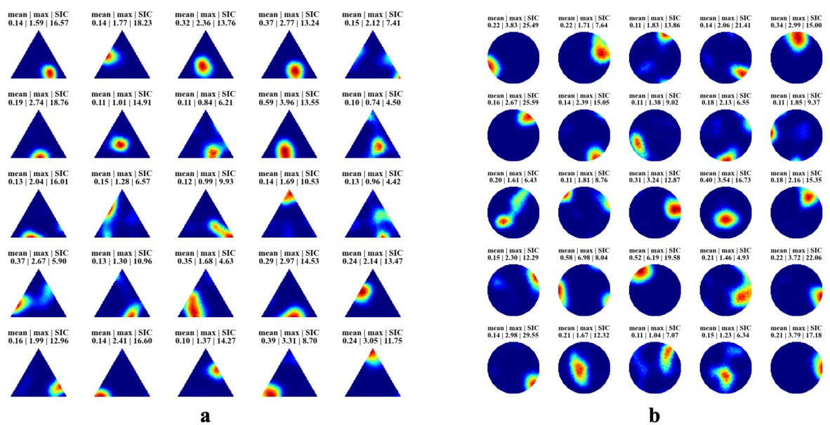
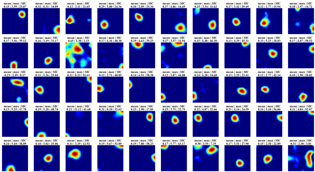
🔼 This figure displays the spatial firing patterns of 40 randomly selected hidden units from the recurrent autoencoder model. Each subplot shows a heatmap representing the firing rate of a single unit across the spatial extent of the simulated environment (a trial room). The color intensity represents the firing rate; higher intensity indicates stronger firing. Many of the units exhibit spatially localized firing patterns, similar to place cells observed in the hippocampus. The mean and maximum firing rates, along with the spatial information content (SIC), are shown for each unit to quantitatively characterize the place-like nature of the responses.
read the caption
Figure 2: Firing maps of 40 randomly selected units in a trial room. A majority demonstrate clear place-like firing patterns. Subplot labels indicate the mean and max firing statistics of each unit in Hz. The spatial information content is indicated in the last column of subplot labels.

🔼 This figure illustrates the concept of experience manifolds (EMs) and how they relate to neuronal firing patterns. Panel a shows an example of an experience manifold created by an agent traversing a 1D track in a 2D experience space. Panels b and c show how two neurons (N1 and N2) with different activation boundaries intersect this manifold, resulting in different firing patterns. Panel d demonstrates remapping: When the agent moves to a new room (EM2), the activity of some neurons might be suppressed temporarily through recurrent inhibition, but is reactivated upon returning to the original room (EM1).
read the caption
Figure 3: a. A room is defined by a unique set of WSM signals describing expected sensory experience at every location. The set of WSM signals converts a room to a hyperplane in experience space. b. Illustration of animal moving from loc1 to loc2 in a 1D track. c. i & iii) Illustration of two neurons N1 and N2 intersecting the experience manifold EM corresponds to the 1D track. ii & iv) Corresponding firing rates as the animal moves from loc1 to loc2. d. EM1 and EM2 are two experience manifolds corresponding to two rooms. The optimal encoding neuron for EM1 may be temporarily inhibited through recurrent connections when entering a new room, then reactivated upon returning to the previous room.
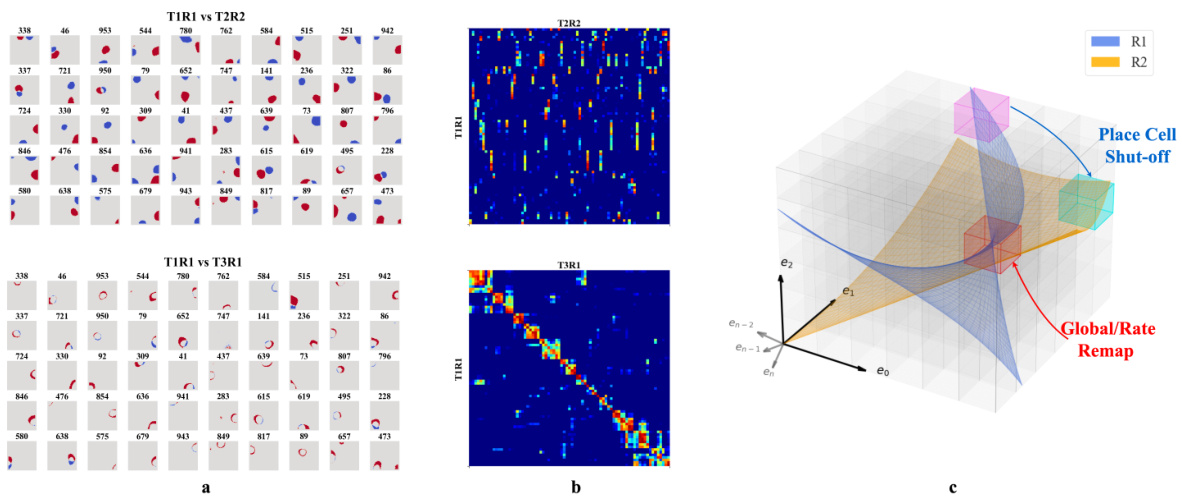
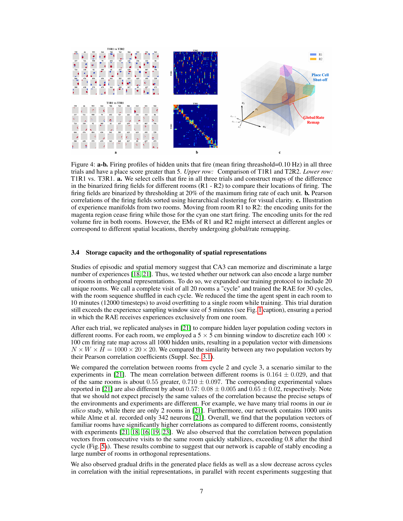
🔼 This figure shows the firing patterns of hidden units in a recurrent autoencoder model trained to simulate episodic memory during spatial navigation. It demonstrates place cell remapping and reversion across different rooms. Panel (a) shows firing maps and Pearson correlation matrices illustrating place field differences between trials in distinct environments. Panel (b) visually represents the results. Panel (c) illustrates how changes in room (experience manifolds) lead to remapping of place cells.
read the caption
Figure 4: a-b. Firing profiles of hidden units that fire (mean firing threashold=0.10 Hz) in all three trials and have a place score greater than 5. Upper row: Comparison of T1R1 and T2R2. Lower row: T1R1 vs. T3R1. a. We select cells that fire in all three trials and construct maps of the difference in the binarized firing fields for different rooms (R1 - R2) to compare their locations of firing. The firing fields are binarized by thresholding at 20% of the maximum firing rate of each unit. b. Pearson correlations of the firing fields sorted using hierarchical clustering for visual clarity. c. Illustration of experience manifolds from two rooms. Moving from room R1 to R2: the encoding units for the magenta region cease firing while those for the cyan one start firing. The encoding units for the red volume fire in both rooms. However, the EMs of R1 and R2 might intersect at different angles or correspond to different spatial locations, thereby undergoing global/rate remapping.
🔼 This figure demonstrates the place cell remapping and reversion phenomena observed in the model. Panels (a) and (b) show firing patterns in different trials (T1R1, T2R2, T3R1) representing different room experiences (R1, R2, R1). Panel (a) visualizes the differences in firing patterns between rooms, showcasing remapping (distinct patterns in different environments). Panel (b) displays a correlation matrix reflecting the similarity between firing patterns, confirming orthogonal representations of the rooms (low correlation between T1R1 and T2R2) and reversion to original patterns when returning to the same room (higher correlation between T1R1 and T3R1). Panel (c) provides a conceptual illustration of experience manifolds (EMs) representing the rooms and how their intersection can lead to remapping.
read the caption
Figure 4: a-b. Firing profiles of hidden units that fire (mean firing threashold=0.10 Hz) in all three trials and have a place score greater than 5. Upper row: Comparison of T1R1 and T2R2. Lower row: T1R1 vs. T3R1. a. We select cells that fire in all three trials and construct maps of the difference in the binarized firing fields for different rooms (R1 - R2) to compare their locations of firing. The firing fields are binarized by thresholding at 20% of the maximum firing rate of each unit. b. Pearson correlations of the firing fields sorted using hierarchical clustering for visual clarity. c. Illustration of experience manifolds from two rooms. Moving from room R1 to R2: the encoding units for the magenta region cease firing while those for the cyan one start firing. The encoding units for the red volume fire in both rooms. However, the EMs of R1 and R2 might intersect at different angles or correspond to different spatial locations, thereby undergoing global/rate remapping.

🔼 This figure demonstrates the robustness of the model to different room shapes and dimensions. Panel (a) shows the emergence of place fields in a 2D environment with two rooms connected by a narrow passage, showing the capability of individual neurons to have multiple place fields in complex environments. Panels (b) and (c) extend this to 3D environments, showing that the model successfully generates 3D place fields with similar properties to those observed in 2D environments. These results highlight the model’s ability to generalize to diverse spatial configurations.
read the caption
Figure 6: a. Example hidden unit firing maps from a model trained in two connected 1m × 1m square rooms. The rooms are connected by a 20cm × 10cm tunnel. b-c To test whether the agent could generate 3D place fields, we assume the agent is able to travel freely in 3D spaces similar to its movement in 2D rooms. We increased the number of WSM channels to 1000 to increase experience specificity in 3D enclosures. b. Placing artificial agents in 3D rooms defined by 3D WSM signals, we observed an emergence of 3D place fields. Locations where neurons fire above 65% max firing rate are densely plotted. 1% of the remaining locations are randomly selected and plotted to indicate neurons firing at these locations. Warmer colors indicate higher firing rates.

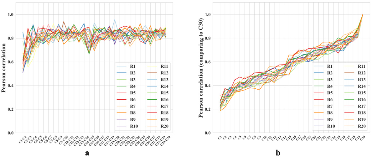
🔼 This figure shows the correlation between population vectors (representing firing patterns of place cells) obtained during trials across 30 cycles. Each cycle included traversing 20 different rooms in a shuffled order. The high correlation along the diagonal shows that the same room’s representation is similar even across different cycles, demonstrating the robustness of spatial representations.
read the caption
Figure 1: Cross correlation of all 600 recorded trials. Each pixel represents a comparison of two trials. During each cycle, the sequence in which the agent explores the 20 rooms is shuffled. We re-organize the room sequence when plotting the cross-correlation between trials to ease visualization. The periodic lines indicate a strong correlation of spatial representations generated when the animals entered the same room, even in different cycles.

🔼 This figure demonstrates the phenomenon of place cell remapping and reversion in the model. Panel (a) shows firing maps for a subset of hidden units across three trials (T1R1, T2R2, T3R1) representing the sequence of navigating two different rooms (R1 and R2). The difference maps highlight changes in firing patterns. Panel (b) presents a correlation matrix of the firing fields, showing low correlation between T1R1 and T2R2 (different rooms) and high correlation between T1R1 and T3R1 (same room, different trial), demonstrating place cell reversion. Panel (c) illustrates how experience manifolds (EMs) from the two rooms interact, providing a conceptual explanation of the remapping mechanism.
read the caption
Figure 4: a-b. Firing profiles of hidden units that fire (mean firing threashold=0.10 Hz) in all three trials and have a place score greater than 5. Upper row: Comparison of T1R1 and T2R2. Lower row: T1R1 vs. T3R1. a. We select cells that fire in all three trials and construct maps of the difference in the binarized firing fields for different rooms (R1 - R2) to compare their locations of firing. The firing fields are binarized by thresholding at 20% of the maximum firing rate of each unit. b. Pearson correlations of the firing fields sorted using hierarchical clustering for visual clarity. c. Illustration of experience manifolds from two rooms. Moving from room R1 to R2: the encoding units for the magenta region cease firing while those for the cyan one start firing. The encoding units for the red volume fire in both rooms. However, the EMs of R1 and R2 might intersect at different angles or correspond to different spatial locations, thereby undergoing global/rate remapping.
🔼 Figure 4 presents the results of an experiment designed to test whether the model supports place cell remapping. The experiment involved training the model on experiences from two different rooms (R1 and R2). Panels (a) and (b) show the firing profiles of hidden units for three trials (T1R1, T2R2, T3R1). Panel (a) shows the differences in the firing fields of units for different rooms, while Panel (b) shows the Pearson correlations of the firing fields. Panel (c) provides an illustration of the experience manifolds from the two rooms, showing how neurons may either cease or begin to fire in different rooms, or shift their firing locations. The figure demonstrates that the model supports key aspects of hippocampal phenomenology, including remapping and reversion.
read the caption
Figure 4: a-b. Firing profiles of hidden units that fire (mean firing threashold=0.10 Hz) in all three trials and have a place score greater than 5. Upper row: Comparison of T1R1 and T2R2. Lower row: T1R1 vs. T3R1. a. We select cells that fire in all three trials and construct maps of the difference in the binarized firing fields for different rooms (R1 - R2) to compare their locations of firing. The firing fields are binarized by thresholding at 20% of the maximum firing rate of each unit. b. Pearson correlations of the firing fields sorted using hierarchical clustering for visual clarity. c. Illustration of experience manifolds from two rooms. Moving from room R1 to R2: the encoding units for the magenta region cease firing while those for the cyan one start firing. The encoding units for the red volume fire in both rooms. However, the EMs of R1 and R2 might intersect at different angles or correspond to different spatial locations, thereby undergoing global/rate remapping.
🔼 This figure demonstrates place cell remapping and reversion in a network trained on experiences from two distinct rooms. Panel (a) displays firing maps highlighting the differences between the firing patterns of the same hidden units in the two rooms, demonstrating remapping by showing some cells only firing in one room and others shifting their firing locations in one room vs the other. Panel (b) shows the correlation between firing patterns, with high diagonal elements when the agent revisits the familiar room showing that spatial representations in the familiar room are preserved. Panel (c) provides an illustration to show the relationship between the concept of experience manifold and how remapping happens in the network. Overall, the results demonstrate the network’s ability to reproduce key aspects of hippocampal place cell phenomenology, including both global and partial remapping and reversion.
read the caption
Figure 4: a-b. Firing profiles of hidden units that fire (mean firing threashold=0.10 Hz) in all three trials and have a place score greater than 5. Upper row: Comparison of T1R1 and T2R2. Lower row: T1R1 vs. T3R1. a. We select cells that fire in all three trials and construct maps of the difference in the binarized firing fields for different rooms (R1 - R2) to compare their locations of firing. The firing fields are binarized by thresholding at 20% of the maximum firing rate of each unit. b. Pearson correlations of the firing fields sorted using hierarchical clustering for visual clarity. c. Illustration of experience manifolds from two rooms. Moving from room R1 to R2: the encoding units for the magenta region cease firing while those for the cyan one start firing. The encoding units for the red volume fire in both rooms. However, the EMs of R1 and R2 might intersect at different angles or correspond to different spatial locations, thereby undergoing global/rate remapping.
🔼 This figure displays the firing patterns of place cells across three trials (T1R1, T2R2, T3R1) in two different rooms (R1, R2). The top row compares trials in R1 and R2, demonstrating remapping (changes in firing patterns), while the bottom row compares trials in R1 across different sessions (R1, R2, R1), demonstrating reversion to original firing patterns after returning to R1. Panel (c) shows a schematic illustrating the relationship between experience manifolds in the two rooms and remapping. The heatmaps illustrate spatial firing patterns, and the correlation matrix shows the similarity between these patterns. This figure demonstrates place cell remapping and reversion, key features of hippocampal place cell activity.
read the caption
Figure 4: a-b. Firing profiles of hidden units that fire (mean firing threashold=0.10 Hz) in all three trials and have a place score greater than 5. Upper row: Comparison of T1R1 and T2R2. Lower row: T1R1 vs. T3R1. a. We select cells that fire in all three trials and construct maps of the difference in the binarized firing fields for different rooms (R1 - R2) to compare their locations of firing. The firing fields are binarized by thresholding at 20% of the maximum firing rate of each unit. b. Pearson correlations of the firing fields sorted using hierarchical clustering for visual clarity. c. Illustration of experience manifolds from two rooms. Moving from room R1 to R2: the encoding units for the magenta region cease firing while those for the cyan one start firing. The encoding units for the red volume fire in both rooms. However, the EMs of R1 and R2 might intersect at different angles or correspond to different spatial locations, thereby undergoing global/rate remapping.
Full paper#
