↗ OpenReview ↗ NeurIPS Homepage ↗ Chat
TL;DR#
Deep neural networks (DNNs) often struggle to learn high-frequency components of functions, a phenomenon known as spectral bias. This bias limits their applicability in many areas dealing with high-frequency data, such as image processing and signal analysis. Existing methods for mitigating spectral bias have shown limited success, especially when dealing with high-dimensional data.
This paper introduces Multi-Grade Deep Learning (MGDL), a novel approach that tackles spectral bias by incrementally learning a function through multiple grades, each grade focusing on low-frequency components. By composing the low-frequency information learned in each grade, MGDL effectively captures high-frequency features. The authors demonstrate MGDL’s efficacy on various datasets, showcasing its ability to overcome the limitations of single-grade methods. MGDL offers a new, effective strategy to address the spectral bias problem, enhancing the performance and generalizability of DNNs in numerous applications.
Key Takeaways#
Why does it matter?#
This paper is crucial because it addresses the spectral bias problem in deep neural networks (DNNs), a significant limitation hindering their performance in tasks involving high-frequency information. By introducing and demonstrating the efficacy of Multi-Grade Deep Learning (MGDL), the research opens new avenues for improving DNN performance and applicability across various fields. The findings are relevant to researchers working on DNNs, high-dimensional data analysis, and applications where high-frequency information is critical.
Visual Insights#

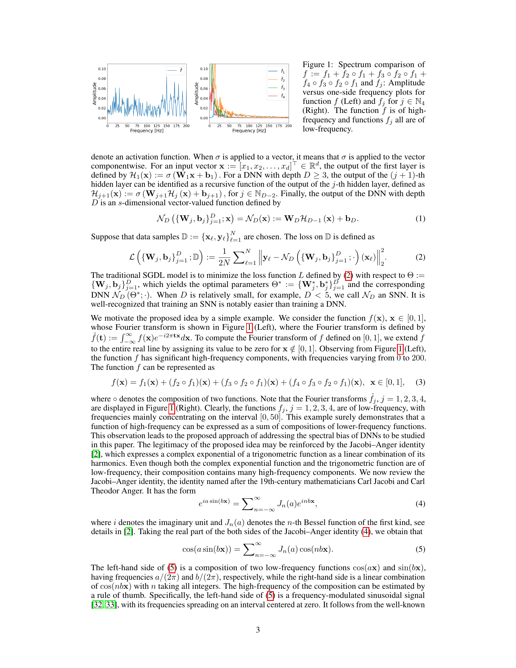
This figure shows the frequency spectrum comparison between a high-frequency function (f) and its four low-frequency components (f1 to f4). The left side shows the spectrum of the high-frequency function f, which is composed of the four low-frequency functions. The right side shows the spectrum of each low-frequency component. This illustrates the concept that a high-frequency function can be represented by composing several low-frequency functions.

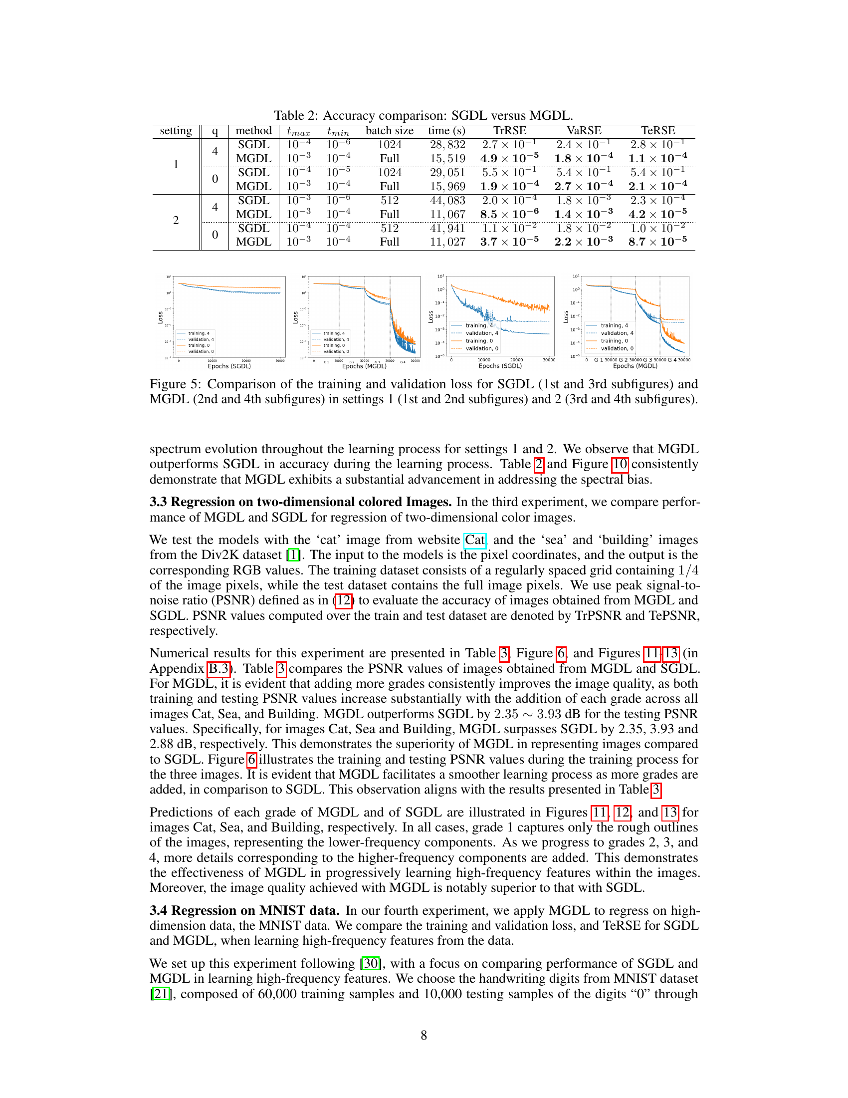
This table compares the performance of Single Grade Deep Learning (SGDL) and Multi-Grade Deep Learning (MGDL) across four different settings. For each setting, it shows the maximum (tmax) and minimum (tmin) learning rates used, the batch size, training time in seconds, and the relative squared error (RSE) on the training, validation, and testing datasets (TrRSE, VaRSE, and TeRSE respectively). The RSE values demonstrate the accuracy of each model, with lower RSE representing higher accuracy. The comparison shows that MGDL achieves significantly lower RSE values across all settings, indicating that it is superior in learning the target functions.
In-depth insights#
Spectral Bias Issue#
The paper focuses on the spectral bias exhibited by deep neural networks (DNNs), where DNNs tend to prioritize learning lower-frequency components of a function while struggling with higher-frequency ones. This bias limits their applicability to problems involving high-frequency information. The authors propose that high-frequency functions can be effectively approximated through the composition of several shallow neural networks (SNNs), each learning low-frequency components. The multi-grade deep learning (MGDL) model is leveraged to implement this idea, learning incrementally, grade by grade, where each grade trains an SNN based on residuals from the previous grade. Experimental results across various datasets show MGDL’s effectiveness in addressing the spectral bias, thereby significantly enhancing the performance and scope of DNNs for applications needing high-frequency representation. MGDL’s efficacy is particularly noticeable in high-dimensional data, demonstrating its potential as a robust solution to a long-standing challenge in deep learning.
MGDL Model#
The MGDL model, a multi-grade deep learning approach, presents a novel strategy for addressing the spectral bias in traditional deep neural networks (DNNs). Unlike standard DNNs that learn all features simultaneously, MGDL decomposes the learning process into sequential grades. Each grade trains a shallow neural network (SNN) focusing on progressively higher frequency components. Crucially, each subsequent grade leverages the low-frequency information extracted by the previous grades as input features. This incremental, compositional approach allows MGDL to effectively capture high-frequency information that often eludes standard DNNs due to their spectral bias towards lower frequencies. The model is inspired by the human learning process, mimicking how complex topics are taught step-by-step building on previously acquired knowledge. The results show that MGDL significantly outperforms traditional methods in various tasks involving high-frequency data, providing a promising solution for improving the performance and applicability of DNNs in diverse domains.
High-Freq Learning#
High-frequency learning in deep neural networks presents a significant challenge due to the spectral bias, where models tend to prioritize lower frequencies. This paper addresses this by proposing a multi-grade deep learning (MGDL) approach. MGDL decomposes the learning process into multiple grades, each focusing on a specific frequency range. Lower frequencies are learned initially in shallower networks, and subsequent grades build upon these, incrementally learning progressively higher frequencies. This compositional approach is inspired by how humans learn complex subjects incrementally through successive grades of education. The efficacy of this method is supported by experimental results on diverse datasets, showing that MGDL effectively captures high-frequency information, while traditional single-grade methods struggle. The key insight is the compositional nature of the learning process, effectively decomposing a complex high-frequency function into manageable components. This technique tackles the spectral bias directly, thus enhancing the performance and expanding the applicability of deep learning models.
Empirical Studies#
In a hypothetical research paper, the ‘Empirical Studies’ section would detail the experiments conducted to validate the proposed approach. This would involve a description of the datasets used, including their characteristics and limitations. Careful consideration of dataset biases is crucial for reliable results. The section should specify the experimental setup, including model architectures, hyperparameters, training procedures, and evaluation metrics. Quantitative results should be presented with appropriate statistical significance measures (e.g., confidence intervals, p-values) to demonstrate the reliability of findings. The authors would compare the proposed approach’s performance against relevant baselines and thoroughly analyze the results, explaining any unexpected findings. Visualizations, such as graphs and charts, would aid in understanding the trends in the results. Finally, a discussion section would reflect upon the findings, acknowledging limitations, and highlighting directions for future research, thereby demonstrating a robust and insightful empirical investigation.
Future Works#
Future research directions stemming from this spectral bias mitigation work could involve developing more robust theoretical foundations for multi-grade deep learning (MGDL). A deeper understanding of MGDL’s convergence properties and its relationship to function approximation theory would enhance its reliability and applicability. Furthermore, exploring alternative architectures and loss functions within the MGDL framework is warranted to further optimize its performance. Investigating the effectiveness of MGDL on a wider variety of high-frequency datasets and complex tasks such as image and video reconstruction or high-dimensional physics simulations is crucial. Finally, analyzing the computational complexity and scalability of MGDL compared to single-grade DNNs would contribute valuable insights for practical applications. Addressing the limitations associated with the reliance on low-frequency components to approximate high-frequency functions within MGDL is important, possibly by investigating alternative decomposition methods.
More visual insights#
More on figures

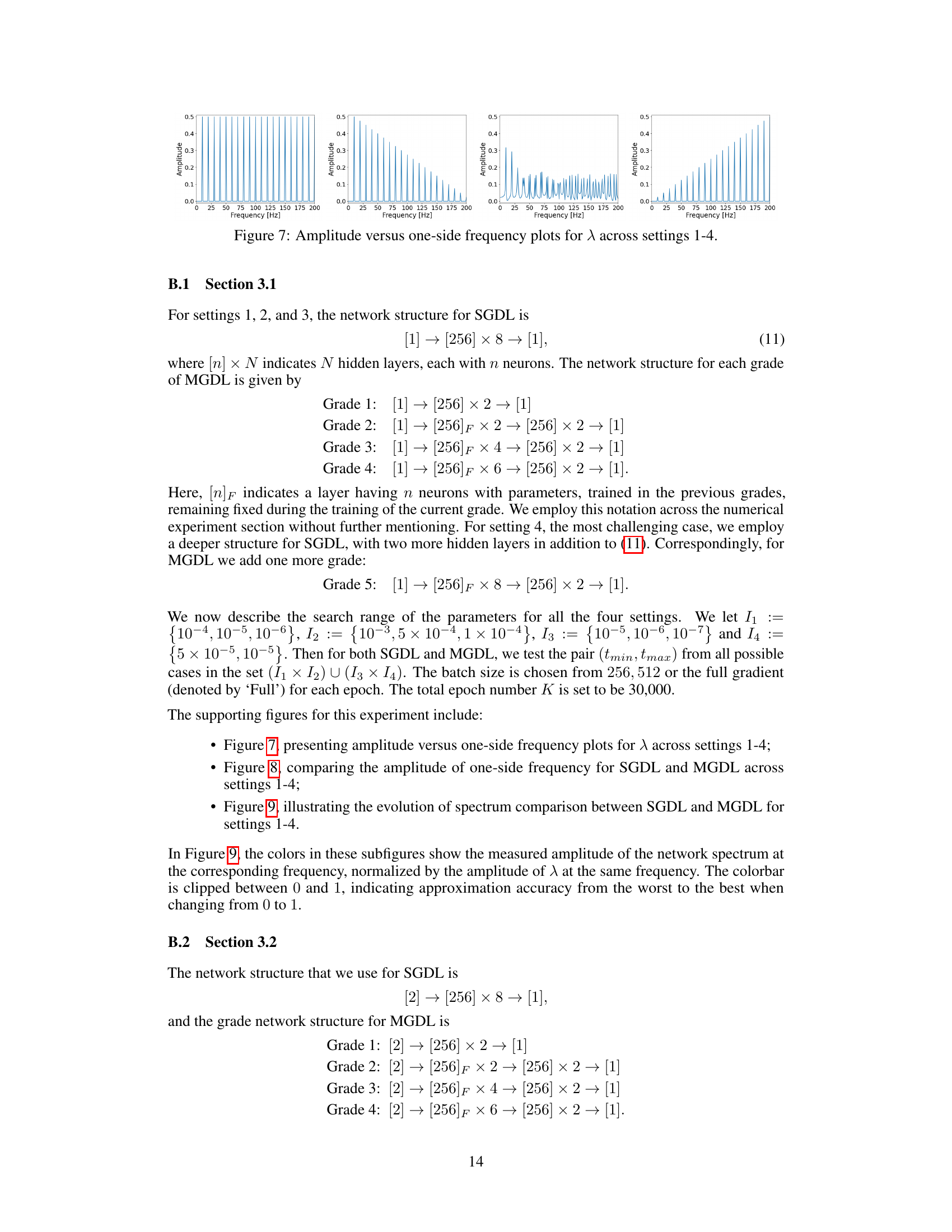
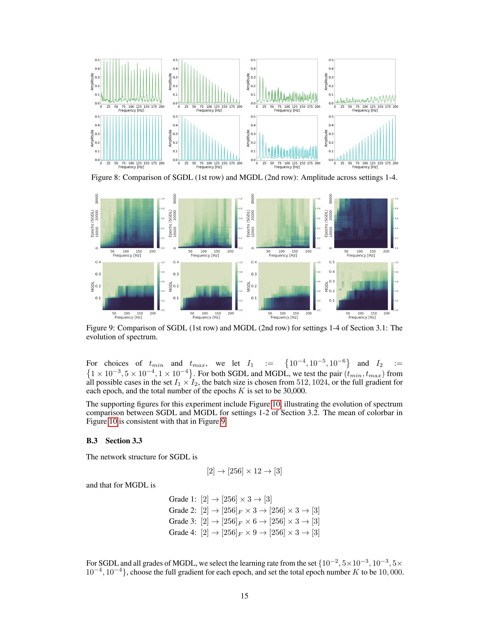
This figure displays the amplitude versus frequency for the functions learned by the Multi-Grade Deep Learning (MGDL) model across four different settings. Each setting represents a different level of complexity in the target function being approximated. The plots show that MGDL learns low-frequency components in the first grade, and progressively learns higher-frequency components in subsequent grades. This demonstrates MGDL’s ability to capture high-frequency information by composing multiple low-frequency components.

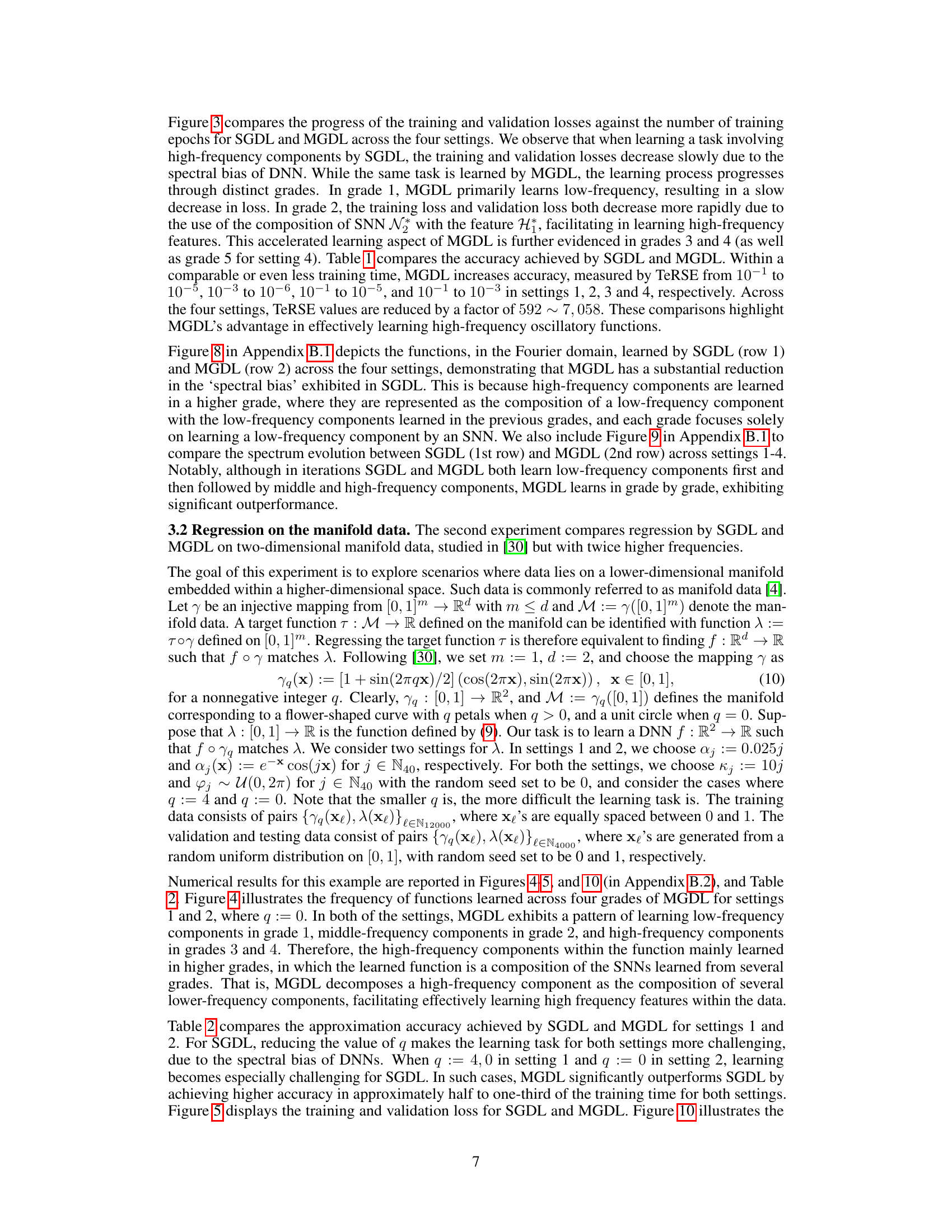
The figure shows the training and validation loss curves for both SGDL and MGDL across four different settings. Each setting represents a different function with varying high-frequency characteristics. The x-axis represents the number of epochs (training iterations), and the y-axis represents the loss (error). The plot highlights how MGDL effectively reduces both training and validation loss compared to SGDL, especially in settings with strong high-frequency components. This demonstrates MGDL’s ability to overcome the spectral bias observed in SGDL and learn high-frequency features more efficiently.

This figure compares the Peak Signal-to-Noise Ratio (PSNR) values for SGDL and MGDL across three different images (Cat, Sea, and Building). Subfigures (a)-(c) show the training and testing PSNR values for SGDL for each image. Subfigures (d)-(f) show the same information for MGDL. The figure illustrates that MGDL achieves higher PSNR values than SGDL, demonstrating that MGDL is better at learning high-frequency features in images.

This figure compares the frequency spectrums of a high-frequency function (f) and its four low-frequency components (f1, f2, f3, f4). The high-frequency function (f) is constructed by the composition of the low-frequency components. The left panel shows the spectrum of f, which has a wide range of frequencies, whereas the right panel shows the spectrums of individual components, which primarily show low-frequency information. This illustrates the paper’s core concept that high-frequency functions can be effectively approximated by the composition of several low-frequency functions.

This figure compares the frequency spectrums of a high-frequency function and its decomposition into several low-frequency functions. The left panel shows the spectrum of the high-frequency function (f), while the right panel displays the spectrums of its individual low-frequency components (fj). This illustrates the core concept of the MGDL method: approximating a complex high-frequency function using simpler, lower-frequency components.
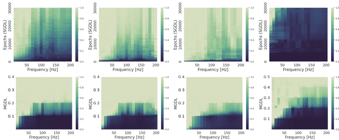
This figure compares the evolution of the spectrum for SGDL and MGDL across four different settings. The top row shows the spectrum for SGDL, while the bottom row shows the spectrum for MGDL. Each column represents a different setting. The colorbar indicates the measured amplitude of the network spectrum at the corresponding frequency, normalized by the amplitude of λ at the same frequency.

This figure compares the evolution of the frequency spectrum learned by SGDL and MGDL across four different settings (1-4) from Section 3.1 of the paper. Each setting represents a different high-frequency function. The top row shows the spectrum learned by SGDL, while the bottom row shows the spectrum learned by MGDL, illustrating how the multi-grade approach captures the high frequencies more effectively through incremental learning.
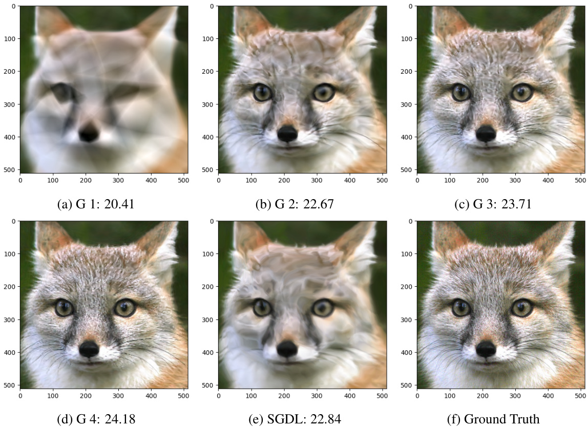
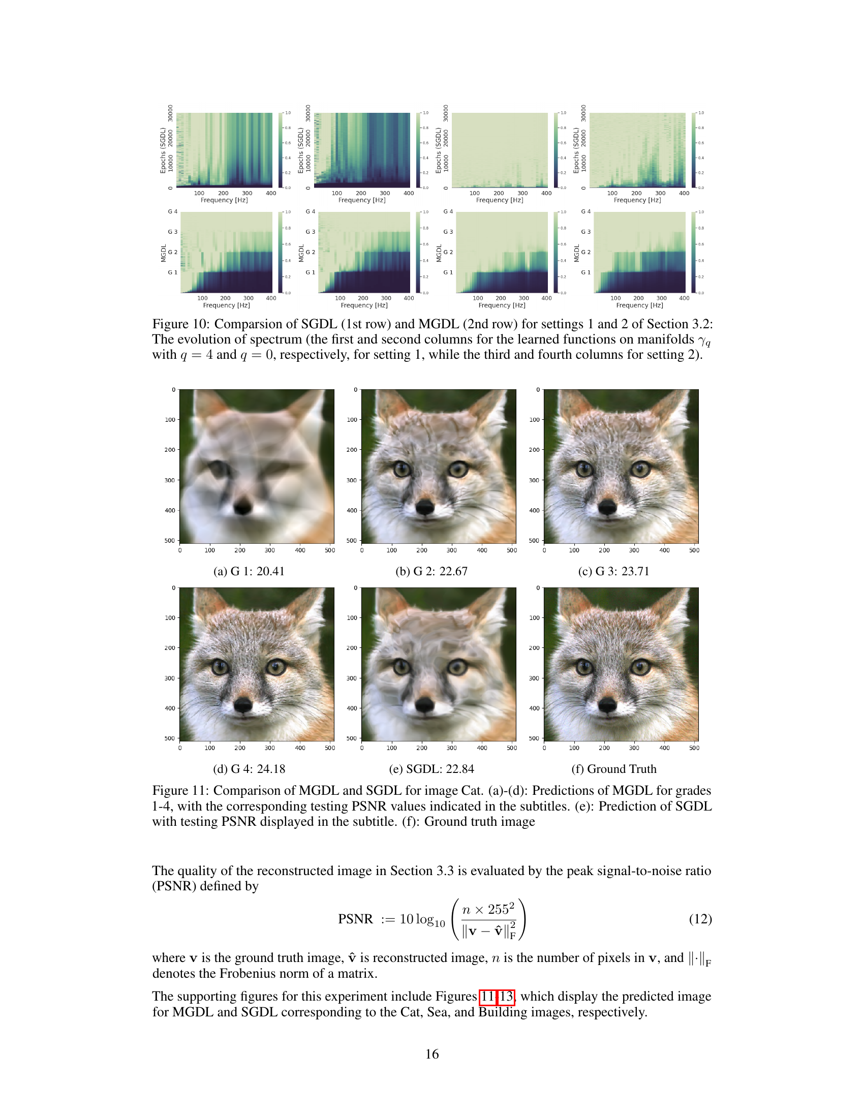
This figure compares the image reconstruction results of MGDL and SGDL on the ‘Cat’ image. MGDL is shown to progressively improve image quality across grades (a-d), achieving higher PSNR values than SGDL (e). The Ground Truth image is provided in (f) for comparison. This demonstrates MGDL’s ability to capture high-frequency details more effectively than SGDL.

This figure compares the frequency spectrums of a high-frequency function (f) and four low-frequency functions (f1 to f4). Function f is constructed as a composition of functions f1 to f4 which demonstrates that high-frequency functions can be constructed by composing lower-frequency functions. This is the core idea of the proposed method that addresses the spectral bias of deep neural networks.
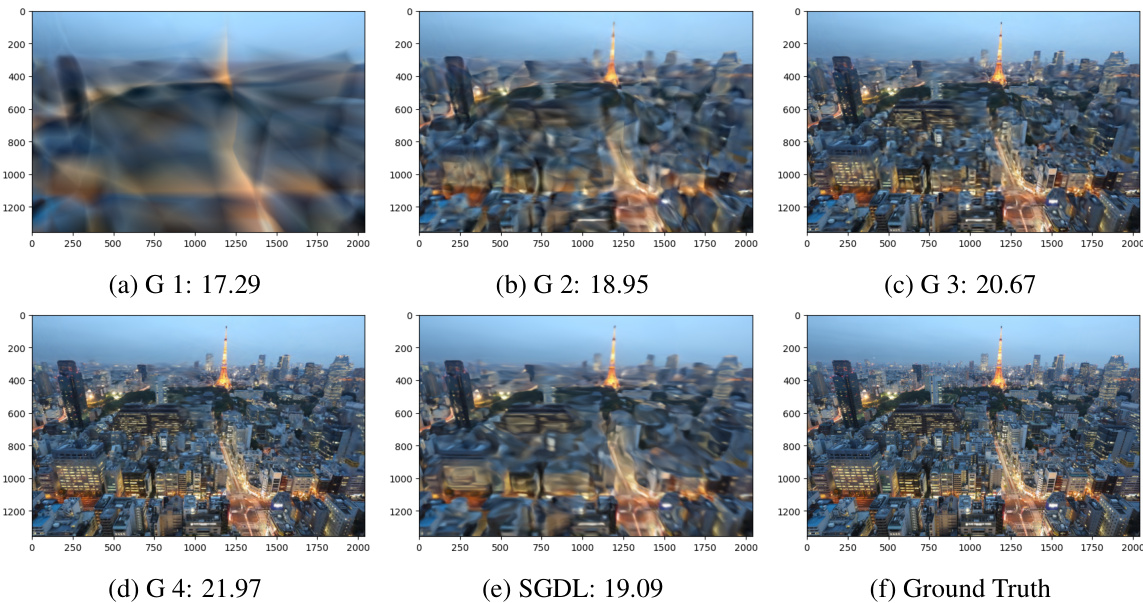
The figure compares the image reconstruction results of the proposed multi-grade deep learning (MGDL) method and the traditional single-grade deep learning (SGDL) method on a ‘Cat’ image. Subfigures (a) through (d) show the results for MGDL across four grades, each grade progressively capturing higher-frequency details, as evidenced by the increasing Peak Signal-to-Noise Ratio (PSNR) values. Subfigure (e) shows the result of SGDL, and subfigure (f) presents the ground truth image. The comparison highlights MGDL’s ability to better capture high-frequency information, leading to improved image quality compared to SGDL.

This figure compares the training and validation losses for both SGDL and MGDL across four different settings. The x-axis represents the number of epochs (iterations of training), while the y-axis represents the loss. It visually demonstrates the faster convergence and lower validation loss achieved by MGDL compared to SGDL, particularly beneficial in settings with high-frequency components.
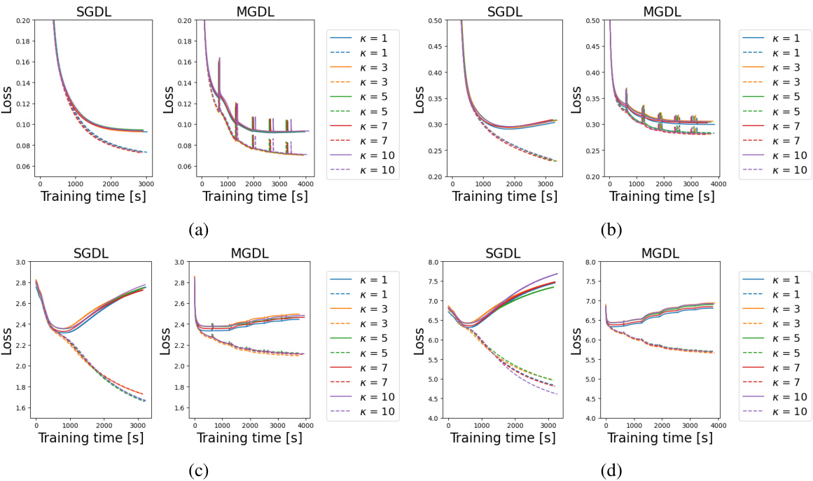
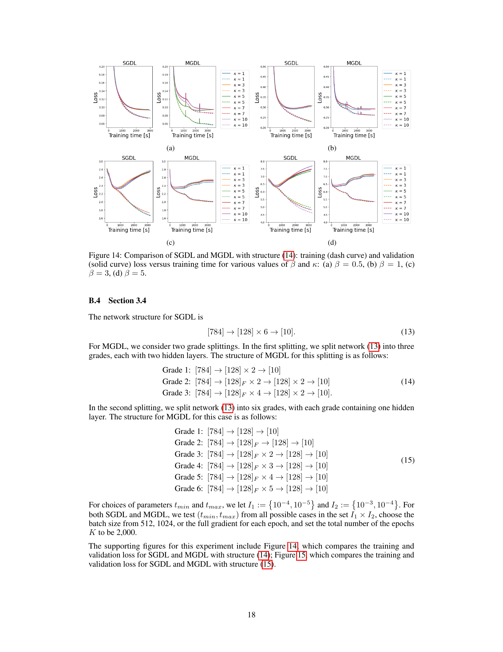
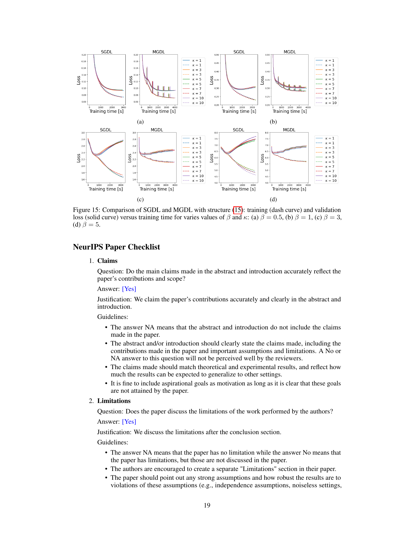
This figure compares the performance of SGDL and MGDL using different structures, focusing on how training and validation loss change over time for various values of amplitude (β) and frequency (κ). Each subplot (a-d) represents a different amplitude level, showcasing how loss changes for both models across various frequencies, providing insights into their learning dynamics in high-frequency scenarios.
More on tables
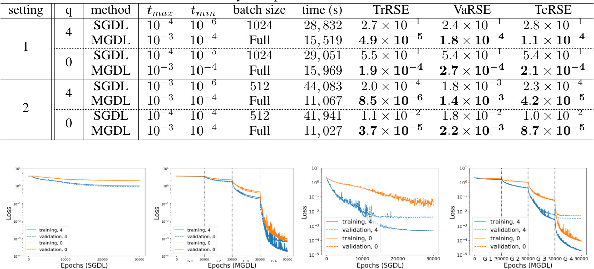
This table presents the results of comparing the performance of SGDL and MGDL in four different settings. Each setting varies the parameters q (related to the complexity of the manifold) and the method used (SGDL or MGDL). The table shows the maximum and minimum learning rates used (tmax, tmin), the batch size, training time, and three relative squared error (RSE) values: training RSE (TrRSE), validation RSE (VaRSE), and testing RSE (TeRSE). These values indicate the accuracy of the models in each setting, with lower values indicating better performance. The results show that MGDL generally outperforms SGDL in terms of testing accuracy, especially in settings with more complex manifolds (q = 0).
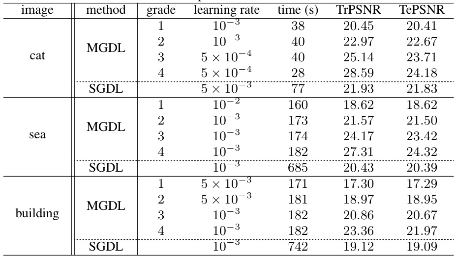
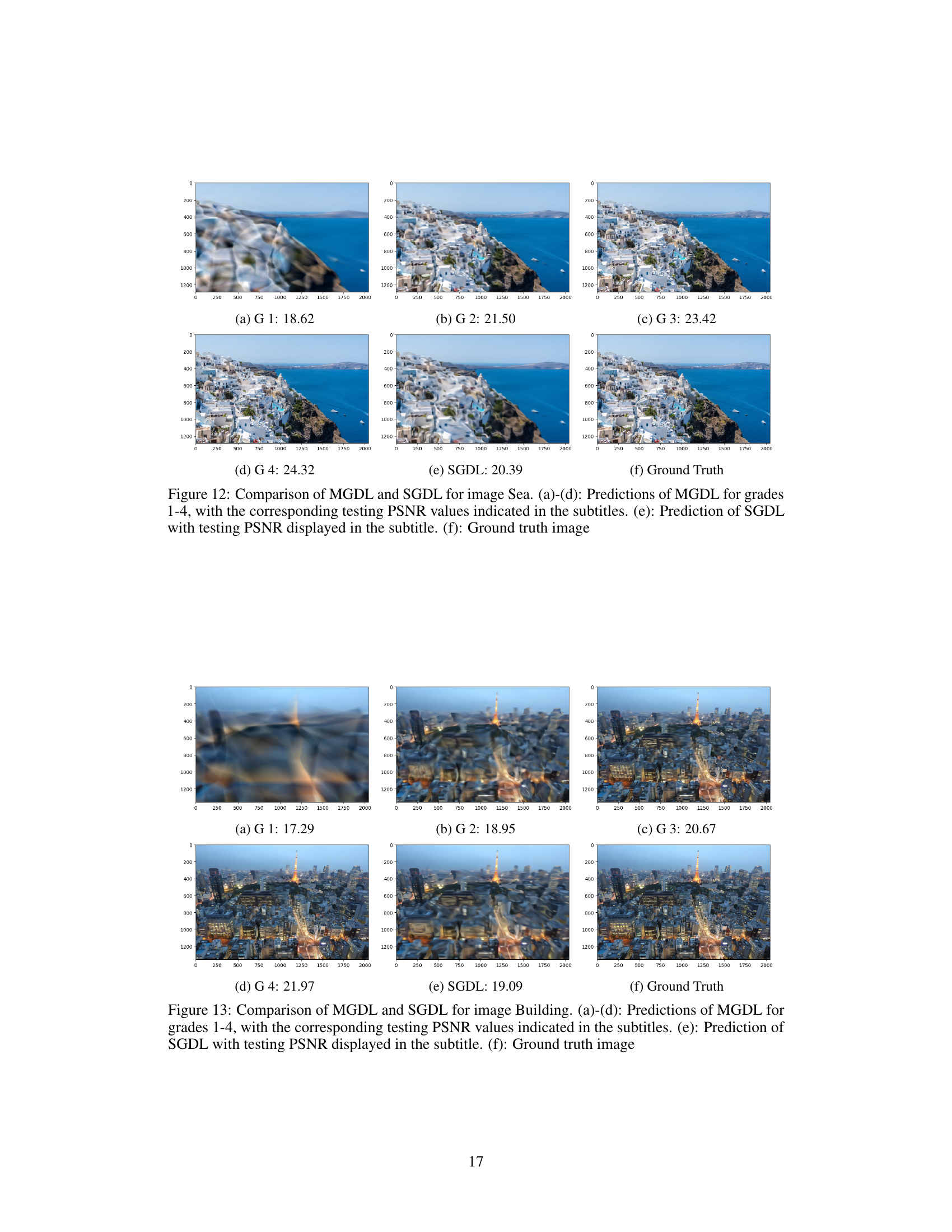
This table presents a comparison of the Peak Signal-to-Noise Ratio (PSNR) values obtained from Single Grade Deep Learning (SGDL) and Multi-Grade Deep Learning (MGDL) for three images: ‘cat’, ‘sea’, and ‘building’. For each image, it shows the PSNR values obtained for both SGDL and MGDL with different numbers of grades (1 to 4 for MGDL). It also indicates the learning rate, training time, training PSNR, and testing PSNR. This allows for a direct comparison of the performance of SGDL and MGDL in image reconstruction tasks, highlighting the benefits of the MGDL approach, particularly in higher grades where high-frequency components are captured.
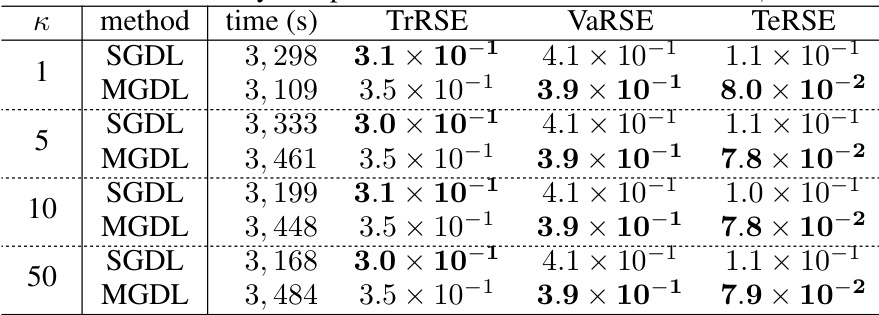
This table presents the comparison of the accuracy of SGDL and MGDL methods for different frequencies (κ) when the amplitude (β) is set to 1. The table shows the training time, training relative squared error (TrRSE), validation relative squared error (VaRSE), and testing relative squared error (TeRSE) for each method and frequency. The results demonstrate the performance of MGDL in achieving lower testing error compared to SGDL, particularly at higher frequencies.
Full paper#

