↗ OpenReview ↗ NeurIPS Homepage ↗ Chat
TL;DR#
Many scientific questions require causal inference from high-dimensional data. Researchers often use machine learning to analyze such data, hoping to estimate causal effects like treatment effects from randomized controlled trials (RCTs). However, this paper theoretically and empirically demonstrates that many common choices in machine learning pipelines can lead to biased estimates of causal effects, even in simple RCT settings. This is because standard machine learning approaches focus on prediction accuracy which is not a proxy for causal inference.
To address these issues, the paper introduces ISTAnt, the first real-world benchmark dataset for causal inference tasks on high-dimensional observations. It uses a study on ant behavior to showcase how various design choices significantly affect the accuracy of causal estimates. A synthetic benchmark is also provided to confirm the results in a controlled environment. The work provides guidelines for designing future benchmarks and representation learning methods to more accurately answer causal questions in the sciences.
Key Takeaways#
Why does it matter?#
This paper is crucial because it reveals significant biases in using machine learning for causal inference in high-dimensional data, a common problem in scientific research. It introduces a novel benchmark dataset and highlights the need for careful design choices in representation learning to avoid misleading conclusions, significantly impacting the reliability of AI-driven scientific discoveries. This work opens avenues for improved methodologies and more robust benchmarks.
Visual Insights#
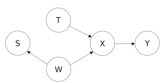
This figure shows a causal graph representing a generic partially annotated scientific experiment. The variables are: T (treatment), W (experimental settings), X (high-dimensional observation), Y (outcome), and S (annotation flag). The arrows indicate causal relationships. For instance, the treatment (T) influences the high-dimensional observation (X), and the observation (X) influences the outcome (Y). The annotation flag (S) is influenced by the experimental settings (W). This model is used to represent the process of estimating the average treatment effect (ATE) in a scenario where annotating the outcome Y for all data points is expensive, so only a subset of data is annotated.

This table shows the Fréchet Distance (FD) between the annotated samples (Ds) and the unannotated samples (Du) for different encoders and annotation splitting criteria. The FD measures the distance between the distributions of feature embeddings from Ds and Du. Higher FD indicates a larger difference in distribution between annotated and unannotated samples, suggesting more spurious correlations between the features and the treatment effect.
In-depth insights#
Causal ATE Bias#
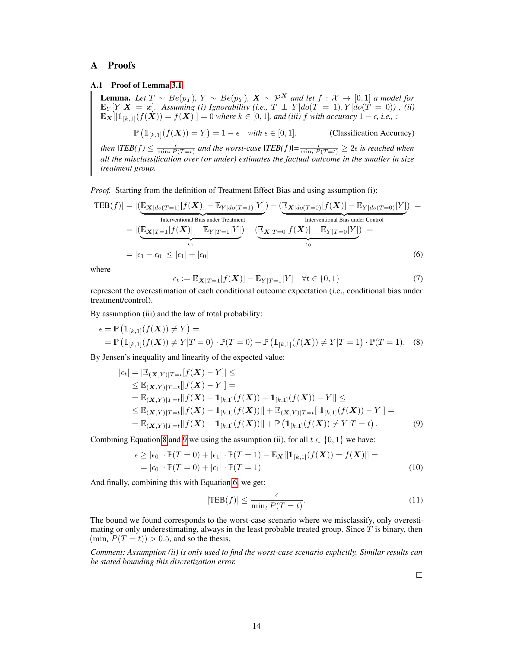
Causal ATE bias refers to the systematic errors in estimating average treatment effects (ATEs) using machine learning models in causal inference. It arises because the model’s predictions, even if accurate in predicting factual outcomes, don’t necessarily translate to accurate causal effect estimates. Several factors contribute to this bias, including data bias (resulting from non-random sampling, e.g., annotating only a subset of the data); model bias (arising from the choice of model architecture, pre-training data, and other model choices); and discretization bias (introduced by thresholding continuous model predictions into binary classifications for ATE estimation). Addressing causal ATE bias requires careful consideration of data sampling techniques, choice of appropriate model architectures, and avoiding unnecessary discretization steps. Proper experimental design, with randomization and appropriate control groups, is also critical. Validation techniques are needed to detect and quantify the bias.
ISTAnt Dataset#
The ISTAnt dataset represents a novel benchmark in causal inference for downstream tasks, specifically focusing on high-dimensional observations within a real-world setting. Unlike existing datasets that primarily utilize simulated or low-dimensional data, ISTAnt uses real-world video recordings of ant behavior, making it more ecologically relevant and challenging. This focus on high-dimensionality necessitates robust representation learning techniques that are evaluated not just on prediction accuracy, but also on their ability to produce accurate and unbiased causal effect estimations. The introduction of a dataset with these characteristics is crucial for advancing research in causal inference and better understanding how it can be applied in real-world scientific problems. The dataset also addresses the bias issue in existing machine-learning-for-science benchmarks by carefully controlling experimental design and incorporating best practices for conducting randomized controlled trials (RCTs). This makes it a valuable tool for researchers to evaluate the impact of various model choices on causal downstream tasks, thereby bridging the gap between AI and the scientific community.
ML Pipeline Bias#
Machine learning (ML) pipelines for causal inference are susceptible to various biases that can significantly distort downstream treatment effect estimations. Data bias, arising from non-random sampling of observations, particularly affects the generalizability of models to unseen data. Model bias emerges from limitations in the representational capacity of the encoder, potentially encoding spurious correlations unrelated to the true causal effect. Discretization bias, introduced by converting continuous model outputs to discrete predictions, further compounds the inaccuracy. The paper emphasizes that standard classification metrics, like accuracy, are insufficient proxies for evaluating the causal validity of ML pipelines. While high accuracy might seem desirable, it does not guarantee accurate treatment effect estimations. A key finding is the recommendation to prioritize the direct estimation of treatment effects using appropriate metrics. This mitigates the misleading effects of prediction-focused evaluation, which ignores the crucial distinction between prediction and causal inference.
Causal Benchmarks#
The concept of “Causal Benchmarks” is crucial for advancing causal inference in machine learning. A good benchmark should not only focus on prediction accuracy but also on the ability of models to accurately estimate causal effects. This requires careful consideration of dataset design, including aspects like the presence of confounding factors, the strength of the causal relationships, and the representativeness of the data. Bias in data collection and annotation significantly affects the reliability of benchmarks, as demonstrated by the various biases highlighted in the provided research paper (sampling, model, and discretization biases). Therefore, developing robust causal benchmarks necessitates not only the use of high-dimensional data from real-world scenarios (like ISTAnt) but also the creation of synthetic datasets (like CausalMNIST) to explicitly control for causal mechanisms. Transparency and open access to data and methods are vital for replicability and validation of results within the field. The effectiveness of established machine learning methods in causal downstream tasks should be rigorously tested and compared on these comprehensive benchmarks to foster progress in the field. The creation of high-quality causal benchmarks is a significant step towards responsible AI development and scientific discovery, where causal understanding is critical.
Future Directions#
Future research should prioritize developing more robust methods for causal inference in high-dimensional settings, addressing the limitations of current deep learning approaches. Improving representation learning techniques to accurately capture underlying causal mechanisms is crucial. This involves exploring alternative architectures, loss functions, and training strategies that are specifically designed for causal discovery. Furthermore, reducing bias in data sampling and model selection is essential. This requires careful consideration of sampling strategies that avoid confounding and adequately represent the population of interest. Developing techniques to quantify and mitigate bias from various sources, such as those introduced by discretization, is a key area. Finally, creating more comprehensive benchmarks for causal downstream tasks, incorporating varied real-world scenarios, will facilitate better evaluation and comparison of causal learning methods, accelerating progress in this vital area of AI research. The creation of synthetic datasets with carefully controlled causal mechanisms would also help in evaluating the efficacy and limitations of different approaches.
More visual insights#
More on figures
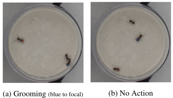
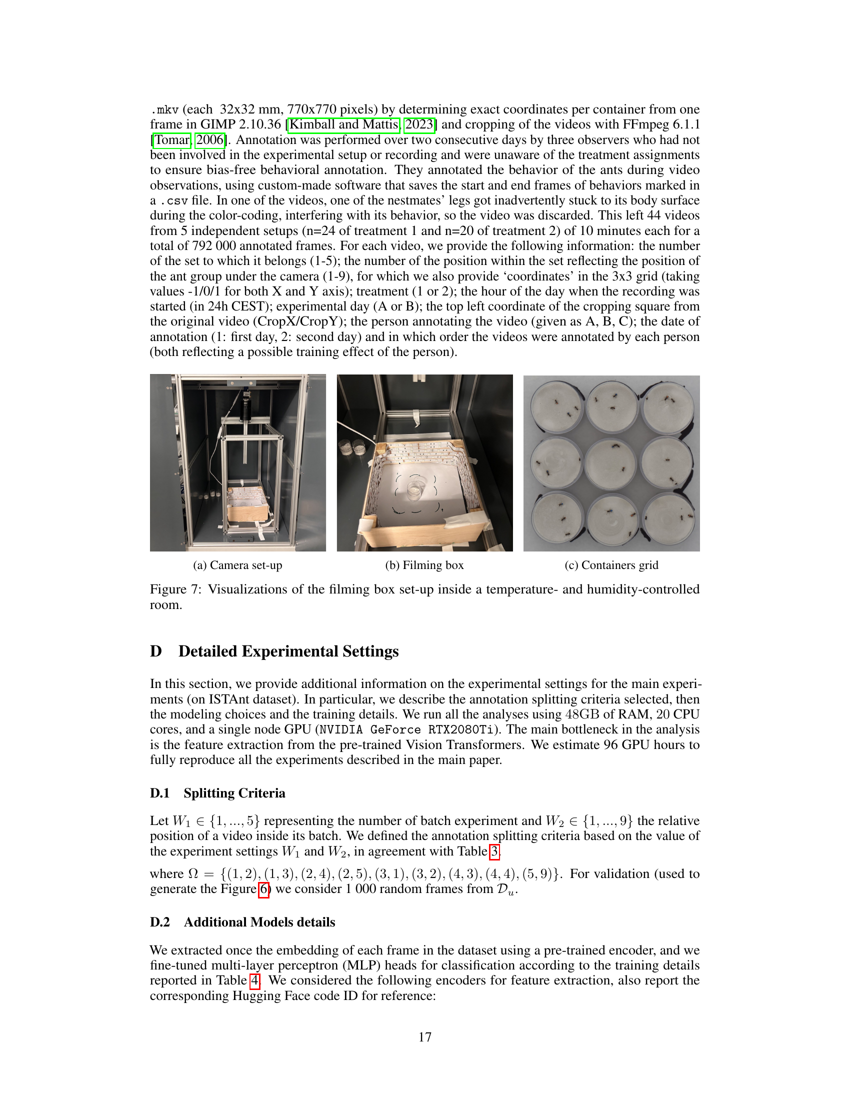
This figure shows two example images from the ISTAnt dataset. The images are high-dimensional observations (X) of ants exhibiting social behavior. The figure visually represents the complexity of the data involved in the study, highlighting the need for sophisticated methods to extract meaningful information for causal inference. (a) depicts ants engaging in grooming behavior (blue ant to focal ant), indicating a positive outcome (Y). (b) depicts ants not engaging in grooming behavior, indicating a negative or null outcome (Y). These images showcase the type of visual data used for the causal inference tasks detailed in the paper.

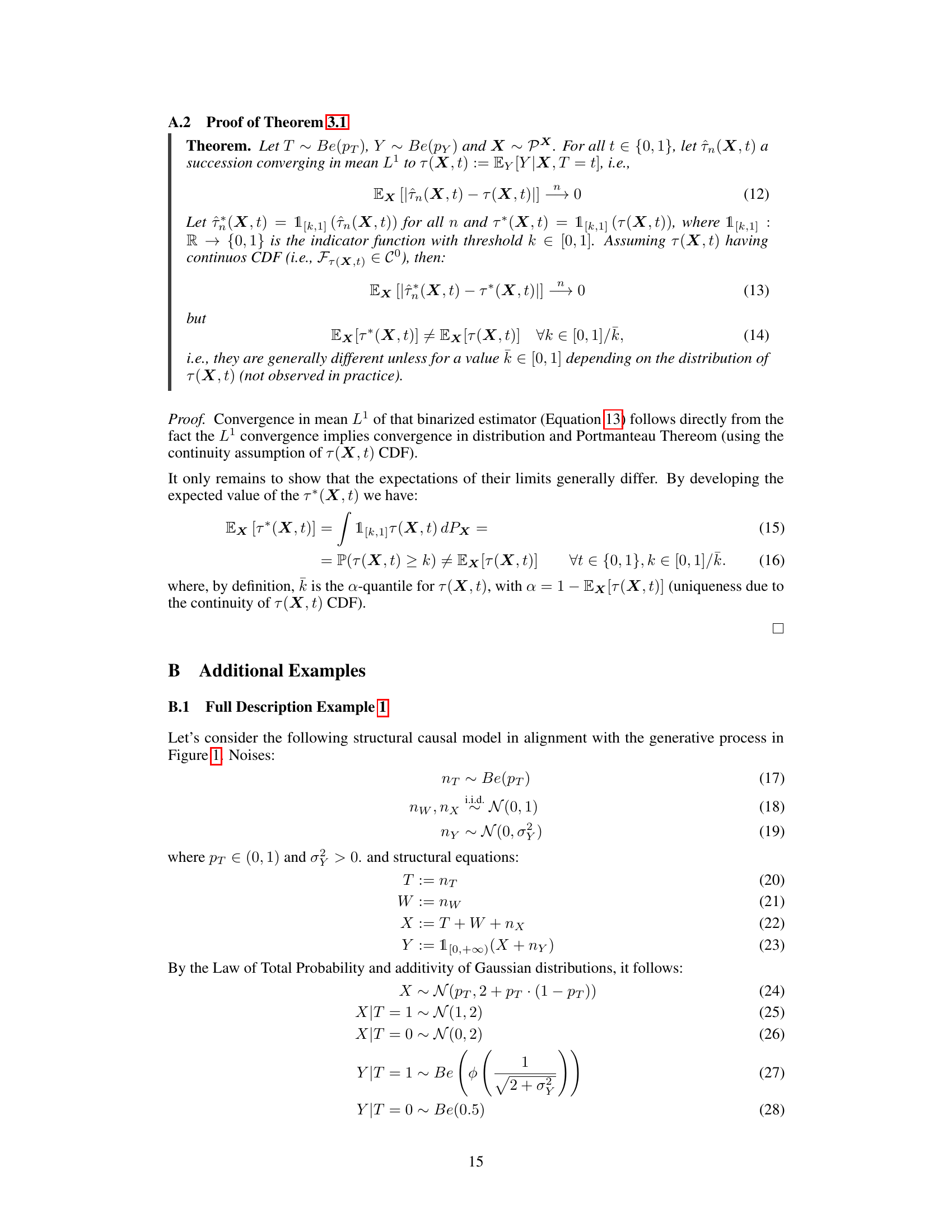
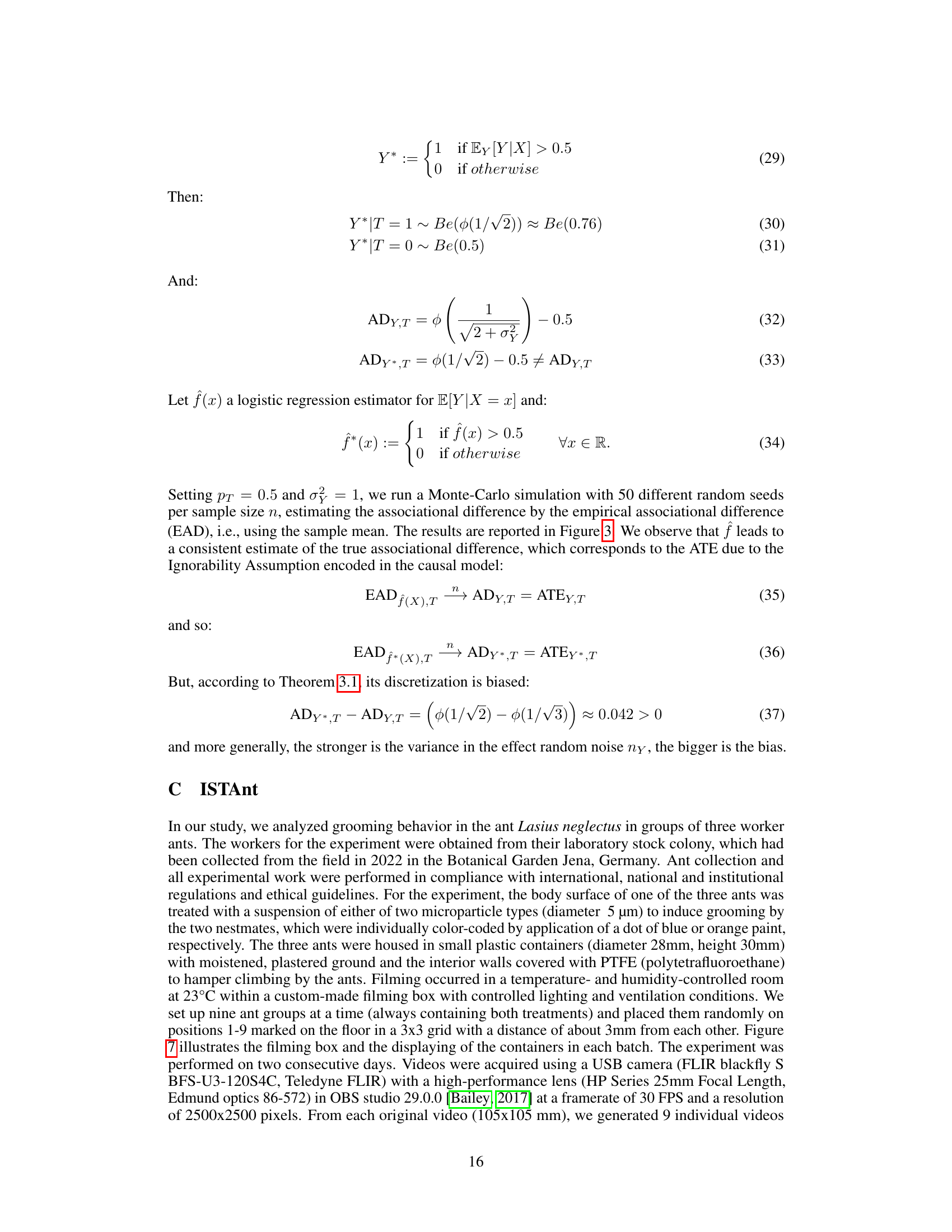
This figure shows the results of a Monte Carlo simulation to illustrate the impact of discretization bias on the estimation of the associational difference. It demonstrates that while a non-discretized model converges to the true associational difference (AD), a discretized version converges to a different, biased value. The degree of bias depends on the randomness in the outcome variable. The figure is used to visually support Theorem 3.1. which shows that discretizing model predictions introduces bias in downstream causal tasks.
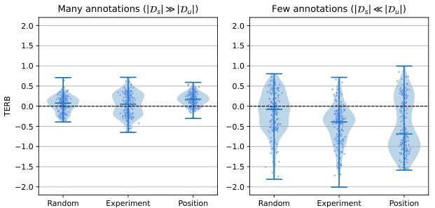
This figure showcases the impact of different annotation criteria (random, experiment-based, position-based) on the Treatment Effect Relative Bias (TERB) when estimating the average treatment effect (ATE). It compares the results for both few-shot and many-shot learning settings. The key takeaway is that biased annotation methods (experiment and position) lead to a significantly biased ATE estimation, while the random annotation method produces a TERB closer to zero, indicating more accurate results.
This figure shows violin plots illustrating the Treatment Effect Relative Bias (TERB) for different annotation criteria in both few-shot and many-shot learning settings. The x-axis represents the annotation criteria (Random, Experiment, Position), while the y-axis shows the TERB. Separate plots are provided for ‘many annotations’ and ‘few annotations’ scenarios, highlighting how the choice of annotation strategy impacts the bias in estimating the average treatment effect. The plots show that the random annotation method leads to less bias compared to the other methods (Experiment, Position), particularly in the few-shot setting. This result supports the paper’s claim that using a biased annotation strategy introduces a bias in the estimation of the causal effect, while random sampling produces more accurate results.
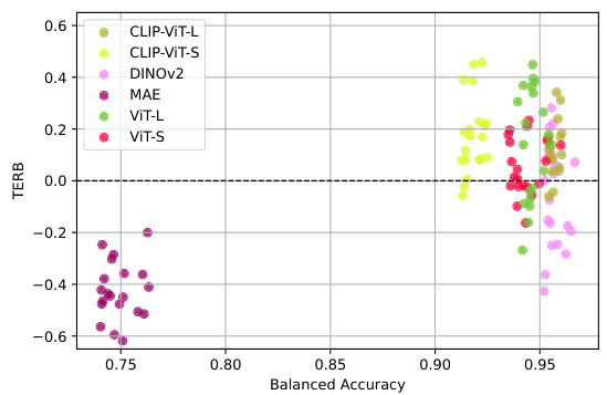
This figure shows a scatter plot illustrating the relationship between the Treatment Effect Relative Bias (TERB) and the balanced accuracy achieved by the top 20 models for each of six different encoders. The x-axis represents balanced accuracy, while the y-axis represents TERB. Each point in the plot represents a model, and the color of each point represents the specific encoder used. The plot demonstrates that even with high balanced accuracy (above 0.95), there’s substantial variation in TERB, ranging from approximately -0.5 to +0.5. This suggests that high predictive accuracy doesn’t necessarily translate to accurate causal effect estimation.

This figure shows the Spearman rank-order correlation between different metrics for model selection. The metrics considered are BCE loss, accuracy, balanced accuracy, and treatment effect bias (TEB) on both validation and full datasets. The results indicate that standard prediction metrics on the validation set have low correlation with the TEB on the full dataset, while the TEB on the validation set shows high correlation with the TEB on the full dataset.

This figure presents a causal model illustrating the relationships between different variables in a generic partially annotated scientific experiment. T represents the treatment, W denotes the experimental settings or conditions, X signifies high-dimensional observations or data, Y is the outcome variable, and S indicates the annotation flag (whether an observation is annotated or not). The arrows in the diagram showcase the causal relationships between these variables.

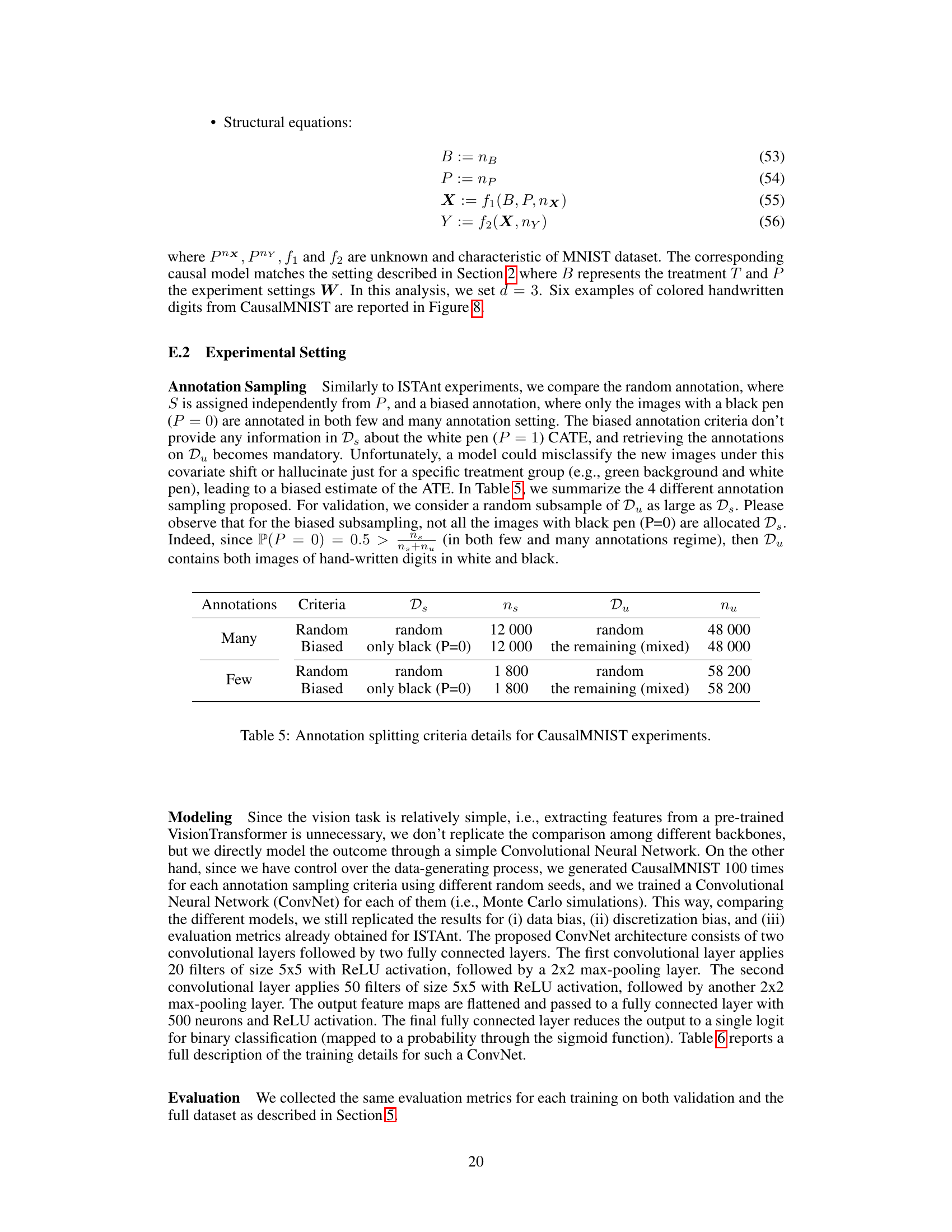
This figure shows six example images from the CausalMNIST dataset. The dataset is a synthetic dataset created by manipulating the MNIST dataset to control for the causal model. The images illustrate how the background color (green or red) and the digit color (white or black) are varied to create different causal effects on the outcome variable Y, representing whether the digit is greater than a threshold value (d). This variation allows researchers to study the impact of different experimental design choices on downstream causal inference tasks.
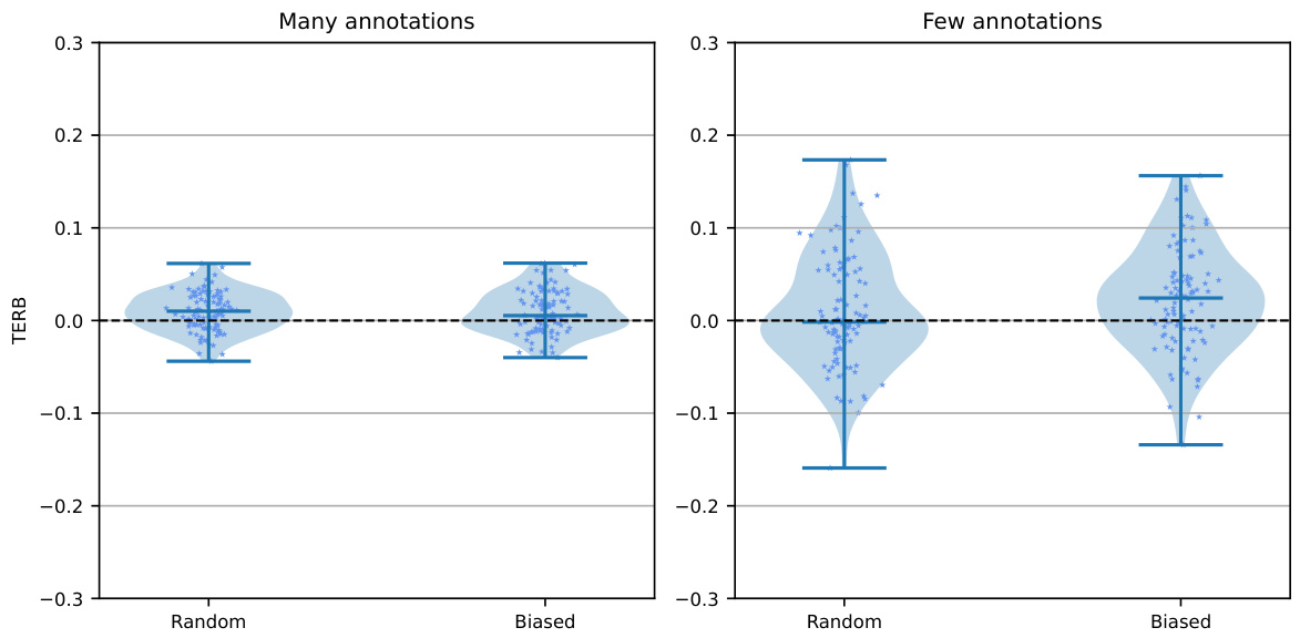
This figure shows violin plots visualizing the Treatment Effect Relative Bias (TERB) for different annotation criteria (random, experiment, position) in both few-shot and many-shot learning scenarios. The plots reveal that biased annotation methods (experiment and position) result in a significantly biased TERB, while random annotation methods yield a TERB closer to zero, indicating unbiased ATE estimation. The results highlight the importance of unbiased sampling techniques in causal inference tasks.
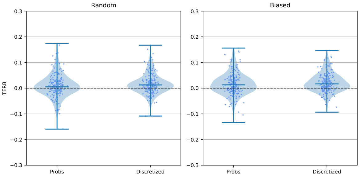
This figure shows violin plots comparing the Treatment Effect Relative Bias (TERB) for models with and without discretization, under both random and biased annotation sampling schemes. The plots are separated into ‘many annotations’ and ‘few annotations’ scenarios to show how the sampling strategy affects bias. The horizontal dashed line represents a TERB of zero (no bias). The plots illustrate that biased annotation generally leads to higher bias than random annotation, and discretization adds extra bias.
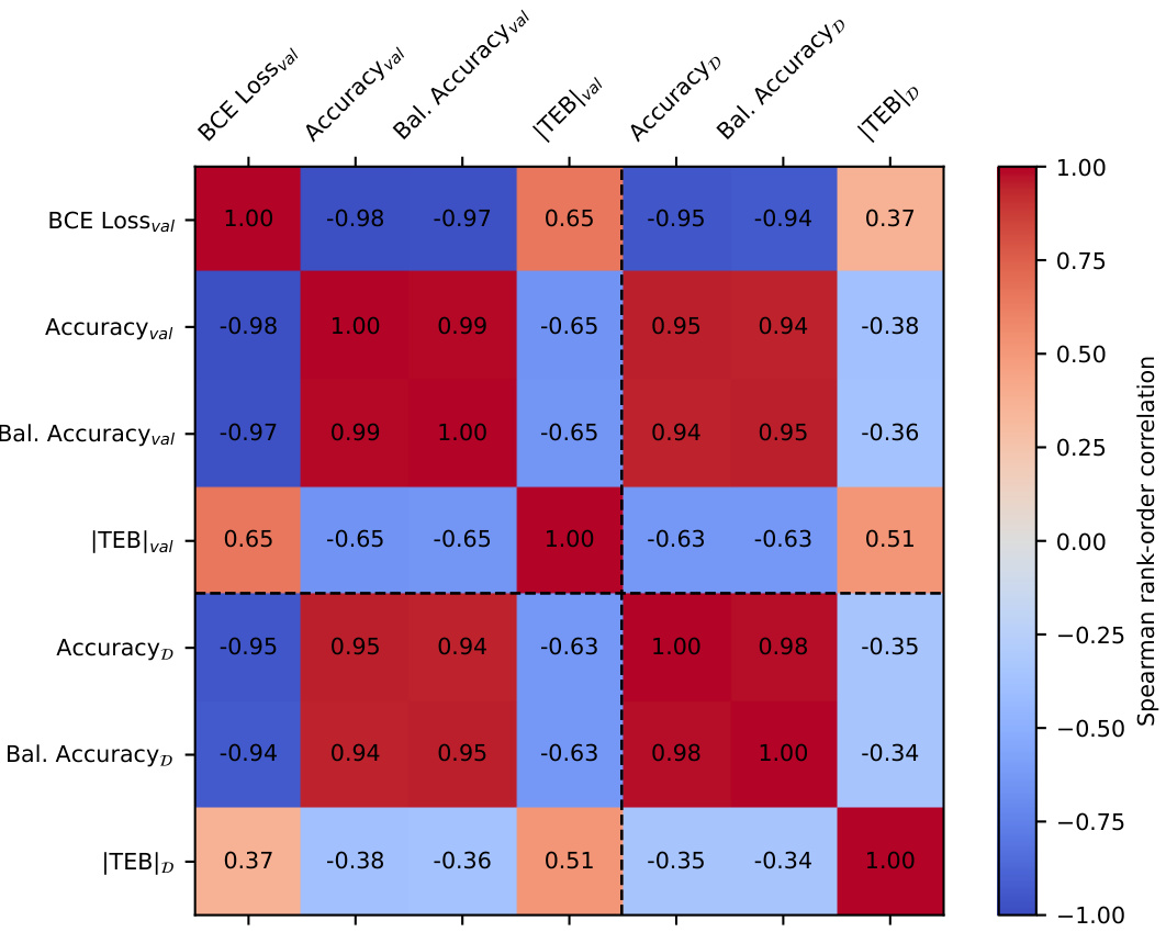
This figure shows the Spearman rank-order correlation matrix between different metrics for model selection. It compares results from validation and the full dataset using 200 models trained with random sampling and varying annotation numbers (few and many). It highlights that while standard prediction metrics correlate well within each dataset, they are less predictive of the treatment effect bias (TEB) on the full dataset. Notably, the TEB from validation is the strongest predictor of TEB on the full dataset.

This figure shows a scatter plot illustrating the relationship between the Treatment Effect Relative Bias (TERB) and balanced accuracy for prediction. The data points represent the top 20 models from six different encoder architectures (ViT-B, ViT-L, CLIP-ViT-B, CLIP-ViT-L, MAE, and DINOv2). It demonstrates that even with high balanced accuracy (above 0.95), the TERB can vary significantly (up to ±50%), indicating that high prediction accuracy doesn’t guarantee accurate causal effect estimation. The exception is MAE, which underperforms other encoders possibly due to focusing on background instead of the ants.
More on tables

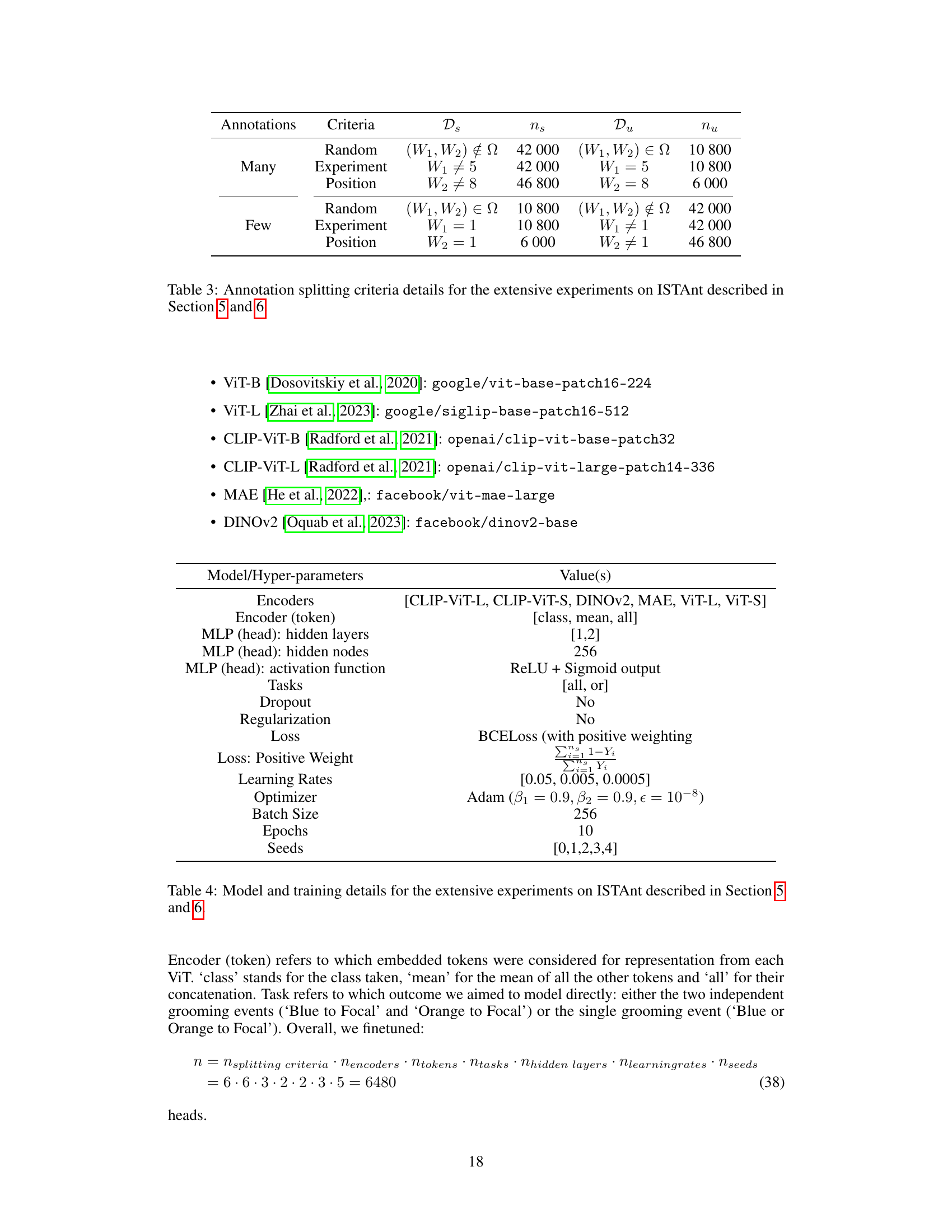
This table details the data splits used in the ISTAnt experiments. Different annotation strategies are compared, each with ‘many’ or ‘few’ annotations. The strategies include random sampling, experiment-based selection (selecting specific batches), and position-based selection (selecting specific positions). For each strategy, the number of samples in the annotated set (Ds) and the unannotated set (Du) are given.

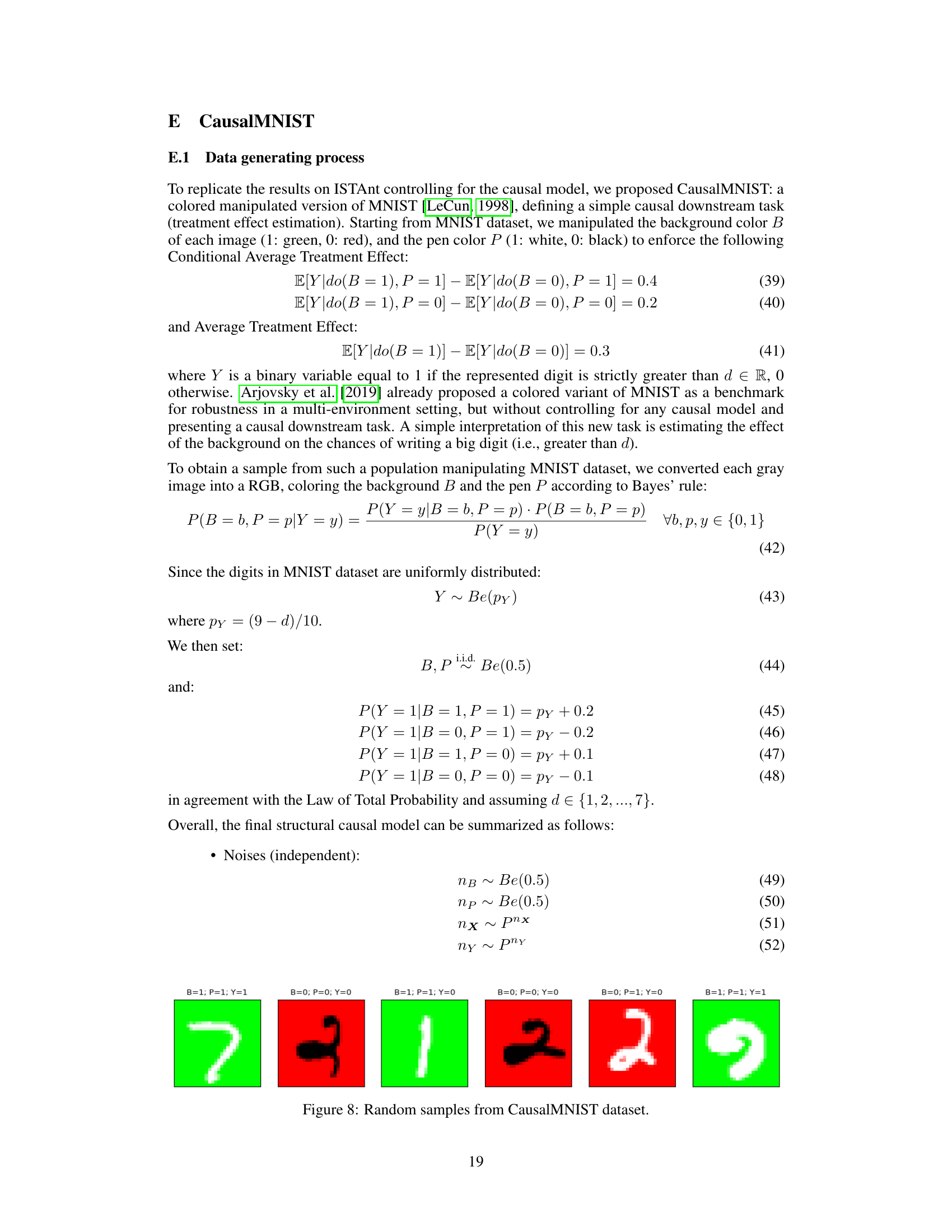
This table details the hyperparameters used in the training of the models for the ISTAnt experiments. It specifies the encoders used (Vision Transformers), the token selection method, the MLP head architecture (number of layers and nodes, activation function), the tasks performed (single or double grooming prediction), whether dropout and regularization were used, the loss function (binary cross-entropy with positive weighting), the learning rates, the optimizer (Adam), batch size, number of epochs, and random seeds used. This information is crucial for reproducibility of the experiments.

This table details the different data splits used in the CausalMNIST experiments. It shows the annotation criteria (random or biased), the number of samples in the annotated set (Ds, ns), and the number of samples in the unannotated set (Du, nu) for both many-shot and few-shot settings. The ‘biased’ criteria annotates only images with a black pen, introducing a potential bias for downstream causal estimations.

This table details the hyperparameters used for training the convolutional neural networks (ConvNets) on the CausalMNIST dataset. It specifies settings such as pre-processing, dropout, regularization, loss function, positive weight for the loss, learning rates, optimizer, batch size, number of epochs, and the number of random seeds used during training.

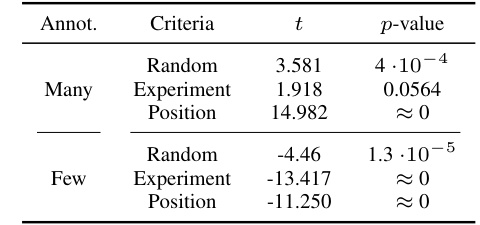
This table presents the results of two-sided t-tests performed to assess the null hypothesis that the treatment effect bias (TEB) of a predictive model (f) is equal to zero. The tests were conducted for different annotation criteria (random and biased) and annotation regimes (many and few annotations). The p-values indicate the statistical significance of rejecting the null hypothesis for each scenario. Small p-values (less than a significance level, e.g., 0.05) suggest strong evidence against the null hypothesis, indicating that the model is likely biased for those conditions.
Full paper#
