TL;DR#
Multimodal learning aims to integrate information from different sources (e.g., audio, text) to get a modality-invariant representation. Classical methods like Canonical Correlation Analysis (CCA) require aligned data, limiting their applicability. Many real-world scenarios involve unaligned data, making shared component identification challenging.
This paper introduces a novel method that tackles this challenge. By minimizing the distribution divergence between different modalities, it can successfully identify shared components from unaligned data under more relaxed conditions than existing methods. This is achieved via adding reasonable structural constraints to address the ambiguity of linear mixture models. This significantly advances the field of multimodal learning and opens new possibilities for various applications.
Key Takeaways#
Why does it matter?#
This paper is crucial because it tackles a core challenge in multimodal learning: identifying shared components from unaligned data. This is highly relevant to many applications like cross-lingual information retrieval and domain adaptation where paired data is scarce or impossible to obtain. The proposed methods and theoretical framework open new avenues for research and development of robust multimodal learning systems.
Visual Insights#

🔼 This figure shows scatter plots of the shared component ‘c’ after applying the proposed method to two different modalities. The left plot corresponds to modality 1, and the right plot corresponds to modality 2. The colors represent the alignment of the data points. Data points of the same color in both plots indicate they are aligned, sharing the same underlying shared component ‘c’. The Gaussian distribution of ‘c’ ensures the data points are clustered appropriately in each plot.
read the caption
Figure 1: Scatter plots of matched distribution (1)c (left) and (2)c (right) when c follows the Gaussian distribution. Colors in the scatter plot represent alignment; same color represent the data are aligned.

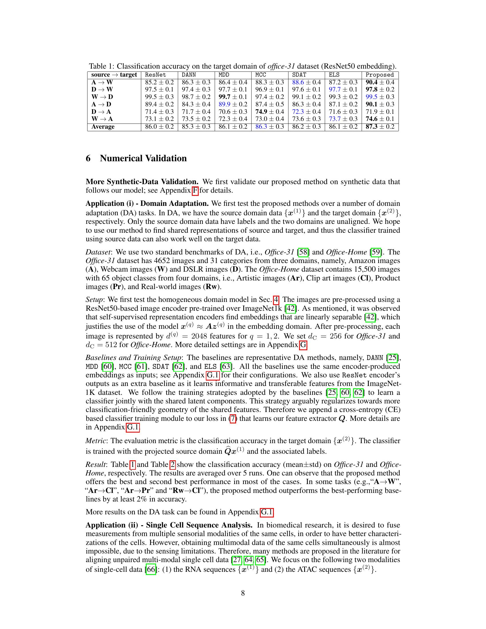
🔼 This table presents the classification accuracy results on the target domain (Office-31 dataset) using ResNet50 embeddings. Different domain adaptation methods are compared: DANN, MDD, MCC, SDAT, ELS, and the proposed method. The results are shown for various source-target domain pairs (A-W, D-W, W-D, A-D, D-A, W-A), along with the average accuracy across all pairs. The table highlights the performance of the proposed method in comparison to existing state-of-the-art domain adaptation techniques.
read the caption
Table 1: Classification accuracy on the target domain of office-31 dataset (ResNet50 embedding).
In-depth insights#
Unpaired Multimodal#
The concept of “Unpaired Multimodal” learning tackles the challenge of integrating information from multiple sources (modalities, e.g., images, text, audio) without the constraint of paired data. This poses a significant hurdle compared to traditional multimodal learning, where corresponding data points across modalities are readily available. The core difficulty lies in establishing meaningful correspondences between unaligned data points from different modalities. Existing methods often rely on techniques like distribution alignment or adversarial learning to find common underlying representations. However, identifiability—the ability to uniquely recover the shared latent factors—remains a key theoretical and practical concern. Research in this area often focuses on deriving sufficient conditions under which identifiability is guaranteed, often involving assumptions about data distributions or the underlying generative process. Successfully addressing unpaired multimodal learning is crucial for various applications where obtaining paired data is impractical or infeasible, opening doors for improved performance in scenarios ranging from cross-lingual information retrieval to medical image analysis.
Shared Component ID#
Analyzing “Shared Component ID” within a research paper necessitates a deep dive into the methodologies used for identifying shared components across multiple modalities. The core challenge lies in disentangling shared information from modality-specific noise. Successful identification relies heavily on the assumptions made about the data generation process; for instance, linear mixture models are common, but their limitations need acknowledging. The identifiability of shared components is often proven under strict conditions, such as statistical independence or specific distribution types for latent variables, and often requires paired or aligned data. The focus on unpaired data significantly increases the difficulty, requiring novel loss functions and careful consideration of distribution discrepancies across modalities. The practical application of these methods hinges on the degree to which the theoretical assumptions hold true for real-world data, and how robust the methods are to violations of these assumptions. Further investigation may explore the impact of dimensionality reduction techniques or the use of alternative modeling frameworks on the accuracy and reliability of shared component identification.
Structural Constraints#
The section on structural constraints explores how additional assumptions, motivated by real-world applications, can significantly improve the identifiability of shared components in unaligned multimodal mixtures. Two key constraints are introduced: homogenous domains and weak supervision. The homogenous domains constraint assumes that both modalities share the same linear mixing system. This simplifies the model and reduces the stringent assumptions necessary for identifiability. The weak supervision constraint, on the other hand, leverages the availability of a few aligned cross-modal samples to further ease identifiability requirements. By incorporating these constraints, the authors demonstrate a considerable relaxation of the conditions needed for successful shared component recovery. This highlights that incorporating prior knowledge about data structure and availability of limited aligned data can dramatically improve the robustness and practicality of unaligned shared component analysis.
Real-World Results#
A dedicated ‘Real-World Results’ section would ideally showcase the model’s performance on diverse, complex real-world datasets, going beyond the controlled environment of synthetic data. This would involve a thorough comparison against established baselines, using relevant evaluation metrics specific to the application domain. Crucially, the section should highlight any unexpected behaviors or limitations observed in real-world settings, contrasting them with the model’s performance on synthetic data. Furthermore, a robust analysis of the results is essential, including error bars or confidence intervals to assess statistical significance. The discussion should offer insightful explanations for any discrepancies between the synthetic and real-world performance, potentially exploring factors like noise, data heterogeneity, or model biases. Detailed descriptions of the real-world datasets used are also key, providing sufficient information for reproducibility. By addressing these aspects, the ‘Real-World Results’ section would convincingly demonstrate the model’s practical applicability and robustness.
Future Directions#
Future research could explore several promising avenues. Extending the theoretical framework to encompass nonlinear multimodal mixtures would significantly enhance the model’s applicability to real-world scenarios where data relationships are complex and non-linear. Investigating the impact of different distribution matching techniques beyond the adversarial approach used in this paper is also crucial. The current approach’s sensitivity to hyperparameter tuning and potential convergence issues warrants further investigation. Developing more robust and efficient algorithms for unaligned shared component analysis, potentially leveraging techniques from optimization and manifold learning, is essential. The identifiability conditions derived are sufficient but not necessary, thus relaxing these conditions would broaden the practical applicability of this work. Finally, empirical evaluations on diverse and large-scale multimodal datasets across various application domains would strengthen the claims and demonstrate broader applicability of this unaligned shared component analysis method.
More visual insights#
More on figures

🔼 This figure validates Theorem 1 presented in the paper, which provides sufficient conditions for identifying shared components from unaligned multimodal linear mixtures. The theorem offers two sets of conditions (a) and (b). The top row shows results obtained using data generated under condition (a), which assumes statistically independent and non-Gaussian content components. The bottom row presents results from data generated under condition (b), which assumes the support of the content component distribution is a hyper-rectangle. In both rows, the scatter plots visualize the learned shared components (represented by color) against the data from each modality. The consistency across conditions (a) and (b) demonstrates that the model effectively identifies shared components under different distributional assumptions.
read the caption
Figure 3: Validation of Theorem 1. Top row: results under assumption (a). Bottom row: results under assumption (b).
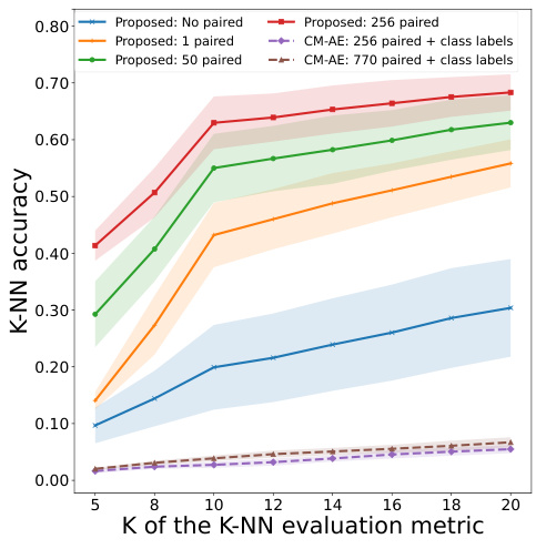
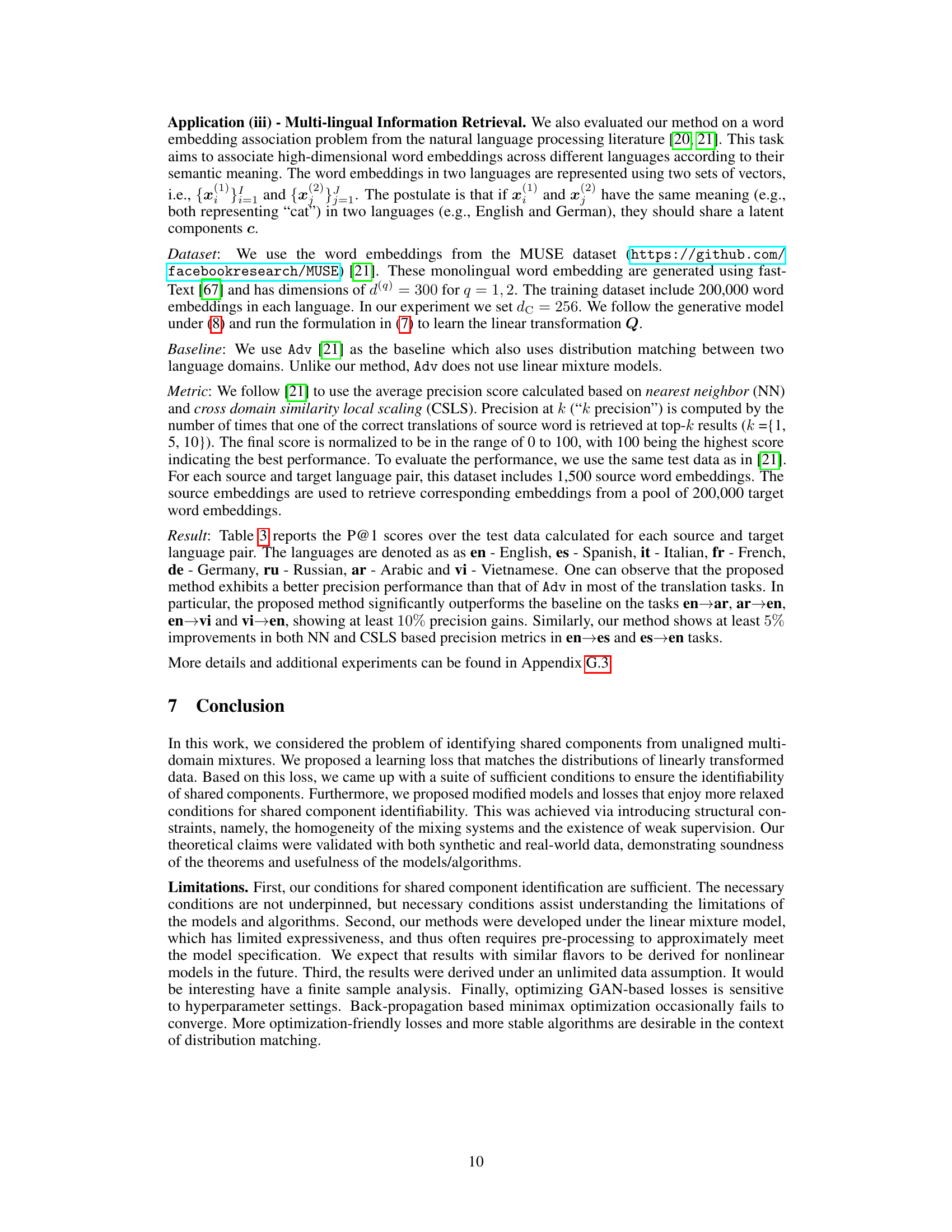
🔼 This figure shows the k-NN accuracy for single-cell sequence alignment using different methods and varying numbers of paired samples. The x-axis represents the value of k in the k-NN evaluation metric, and the y-axis shows the corresponding accuracy. The plot compares the performance of the proposed method with and without weak supervision (different numbers of paired samples) against a baseline approach (CM-AE). Error bars are included to show the variation in the results.
read the caption
Figure 4: k-NN accuracy for single-cell sequence alignment.

🔼 This figure shows the results of a numerical validation for Theorem 3. The experiment varies the number of aligned cross-domain samples (anchors) used in the unaligned shared component analysis (SCA) problem. The top row displays the 2D t-SNE visualization of the shared component c obtained under different conditions: ground truth, no anchors, 1 anchor, and 3 anchors. The bottom rows show the corresponding 2D t-SNE visualizations of the private components p(1) and p(2) for each modality. The black crosses in the plots mark the centroids of each cluster. The results demonstrate that the proposed method effectively identifies the shared component when enough aligned samples are available, which is consistent with Theorem 3.
read the caption
Figure 5: Validation of Theorem 3: dc = 3 and dp = 1.

🔼 This figure visualizes the results of applying t-SNE to reduce the dimensionality of features extracted from the Office-31 dataset using CLIP and the proposed method. The left panel shows the original CLIP features (768 dimensions), demonstrating some clustering by class but significant overlap. The right panel shows the lower-dimensional (256 dimensions) features produced by the proposed method. The improved separation of classes in the right panel illustrates the effectiveness of the proposed method in enhancing the discriminability of the data.
read the caption
Figure 6: Office-31 dataset: DSLR images features represented as circle markers, Amazon images features represented as triangle markers. Different color represent different classes.
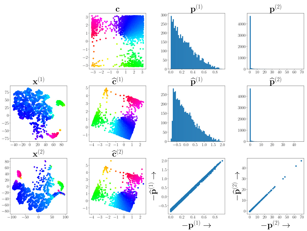
🔼 This figure validates Theorem 1 presented in the paper, which provides conditions for identifying shared components from unaligned multimodal linear mixtures. The top row shows results obtained under assumption (a) of the theorem, where the individual elements of the shared components are statistically independent and non-Gaussian. The bottom row displays results under assumption (b), where the shared components follow a hyper-rectangular distribution. Each plot visually represents the learned shared components against the true shared components, demonstrating that the proposed method accurately recovers the shared components under the specified conditions.
read the caption
Figure 3: Validation of Theorem 1. Top row: results under assumption (a). Bottom row: results under assumption (b).
More on tables

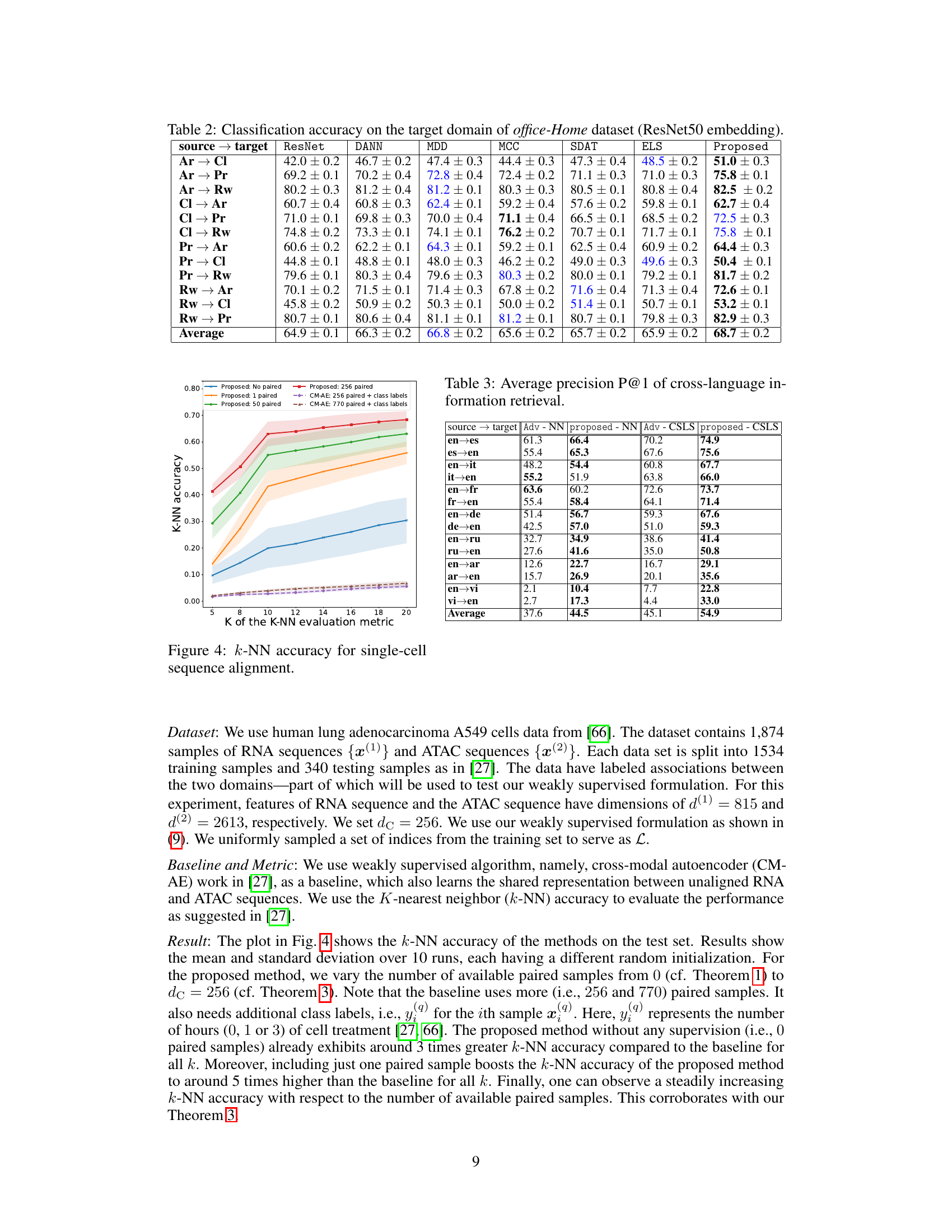
🔼 This table presents the classification accuracy results on the Office-Home dataset’s target domain. The ResNet50 embedding is used as input features. Different domain adaptation methods (DANN, MDD, MCC, SDAT, ELS, and the proposed method) are compared, showing the average accuracy and standard deviation across various source-to-target domain transfer tasks (Ar→Cl, Ar→Pr, Ar→Rw, Cl→Ar, Cl→Pr, Cl→Rw, Pr→Ar, Pr→Cl, Pr→Rw, Rw→Ar, Rw→Cl, Rw→Pr).
read the caption
Table 2: Classification accuracy on the target domain of office-Home dataset (ResNet50 embedding).
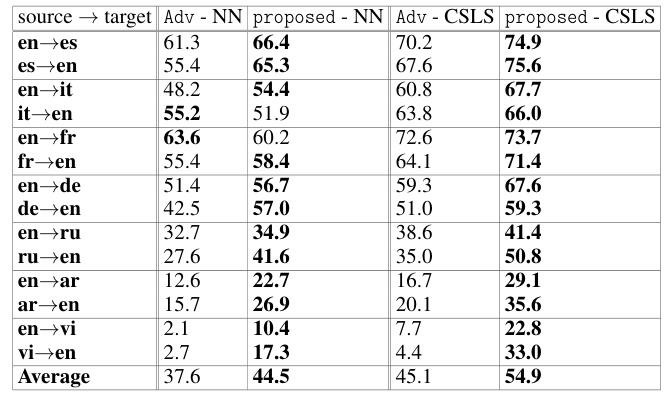
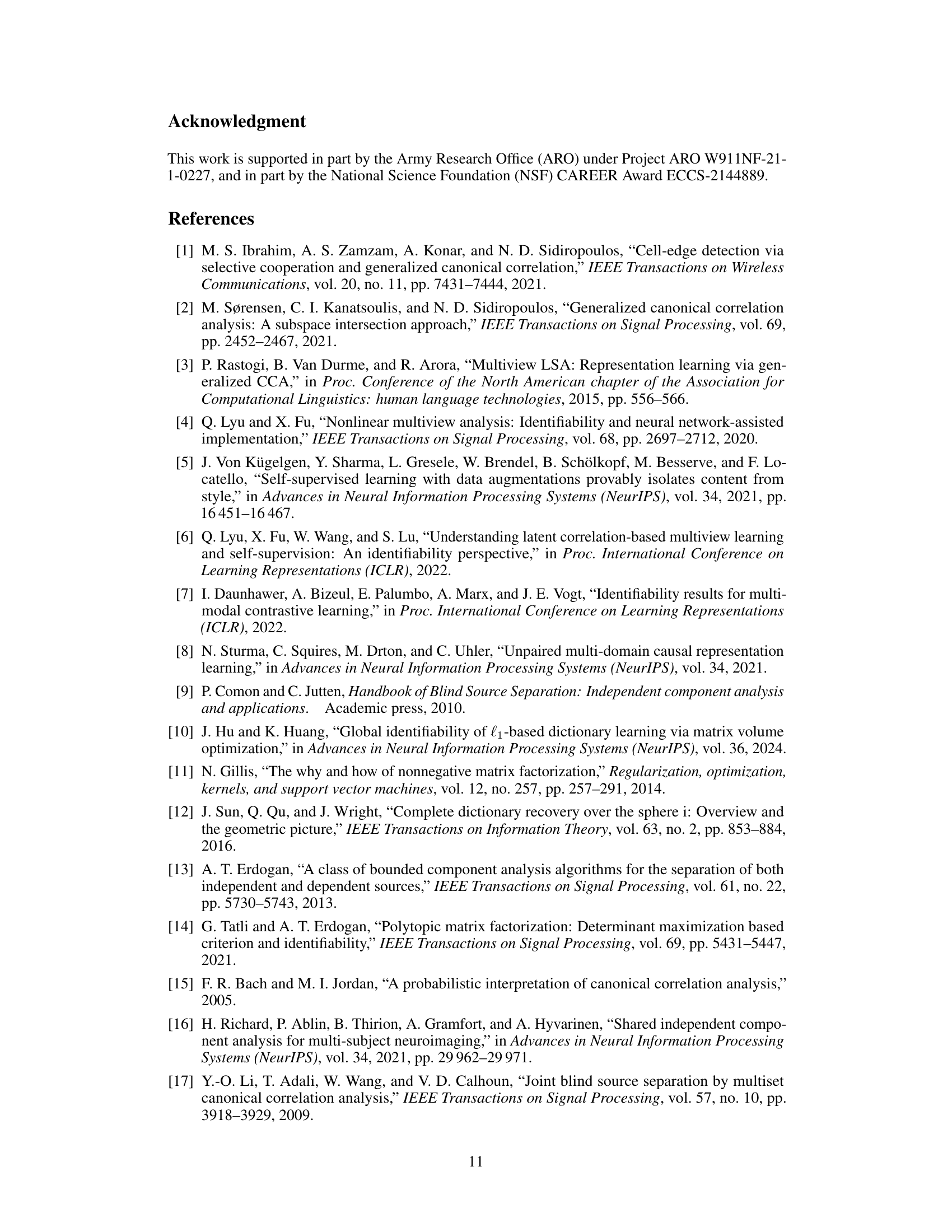
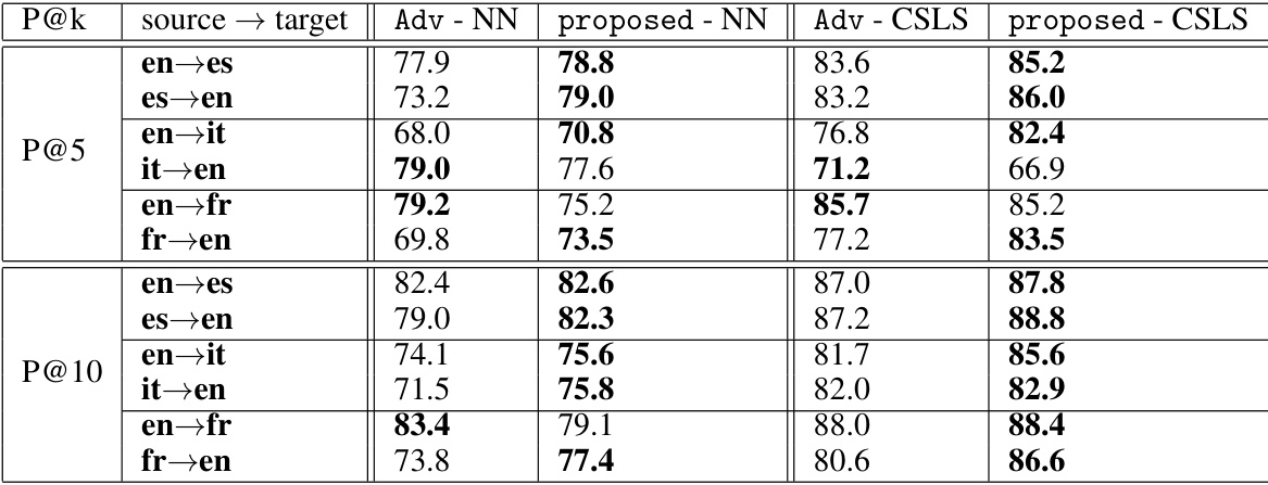
🔼 This table presents the average precision at rank 1 (P@1) for cross-language information retrieval, comparing the proposed method against a baseline (Adv). The results are broken down by language pairs (e.g., en-es for English to Spanish, es-en for Spanish to English), showing the performance using both nearest neighbor (NN) and cross-domain similarity local scaling (CSLS) methods. The average P@1 scores across all language pairs are also provided.
read the caption
Table 3: Average precision P@1 of cross-language information retrieval.
🔼 This table presents the classification accuracy results for domain adaptation experiments using the Office-31 dataset. The ResNet50 embedding is used as the image feature. The table shows the accuracy of different domain adaptation methods (DANN, MDD, MCC, SDAT, ELS, and the proposed method) for various source-target domain pairs (A-W, D-W, W-D, A-D, D-A, W-A). The results highlight the performance of each method on different cross-domain tasks, indicating its effectiveness in transferring knowledge from source to target domains.
read the caption
Table 1: Classification accuracy on the target domain of office-31 dataset (ResNet50 embedding).

🔼 This table presents the results of a numerical experiment conducted to validate Theorem 1 under different sample sizes. It shows the performance of Shared Component Analysis (SCA) and Canonical Correlation Analysis (CCA) in identifying shared components when the number of samples (N) varies from 100,000 to 20. Two metrics are used to evaluate performance: the Frobenius norm of the difference between the estimated linear transformations of the two modalities, and a second metric that measures how well the private components are discarded in the low dimensional space. The results indicate that the SCA method effectively identifies shared components even when the sample size is small, while CCA’s performance is less robust.
read the caption
Table 5: Shared component identification performance over different N.

🔼 This table presents the results of experiments evaluating the performance of shared component identification under different sample sizes in the two modalities. The number of samples in the first modality is held constant at 100,000, while the number of samples in the second modality is varied (10,000, 1,000, 100, and 10). The table shows two key metrics: the Frobenius norm of the difference between the estimated shared components from the two modalities, and the average Frobenius norm of the private components across the two modalities. Smaller values for both metrics indicate better performance in identifying the shared components.
read the caption
Table 6: Shared component identification performance under imbalanced multi-modal data sizes.
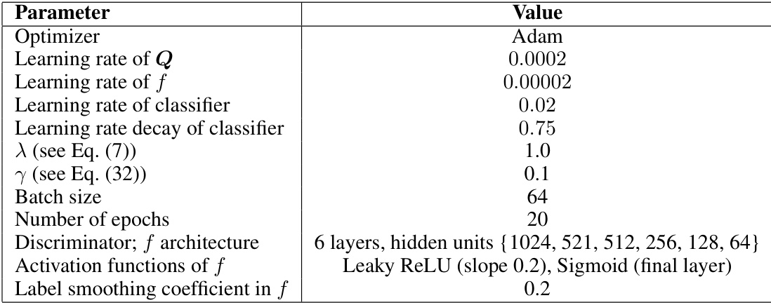
🔼 This table lists the hyperparameters used in the domain adaptation experiments. The optimizer used is Adam. Learning rates are specified for the Q matrices, discriminator f, and the classifier, along with a decay rate for the classifier learning rate. Lambda and gamma are parameters from the loss functions, the batch size, and number of epochs are also indicated. The discriminator’s architecture is detailed, showing a 6-layer MLP with specified hidden units and activation functions (leaky ReLU and sigmoid). Finally, a label smoothing coefficient is given.
read the caption
Table 7: Hyperparameter settings for domain adaptation.

🔼 This table presents the classification accuracy results for the Office-31 dataset’s domain adaptation task using ResNet50 embeddings. It compares the proposed method against several baselines (DANN, MDD, MCC, SDAT, ELS) across different source-target domain combinations (A-W, D-W, W-D, A-D, D-A, W-A). The accuracy is reported as a mean ± standard deviation, showcasing the performance of each method in transferring knowledge from the source domain to the target domain.
read the caption
Table 1: Classification accuracy on the target domain of office-31 dataset (ResNet50 embedding).

🔼 This table presents the classification accuracy results for domain adaptation experiments using the Office-31 dataset and ResNet50 embeddings. It compares the performance of the proposed method against several existing domain adaptation techniques (DANN, MDD, MCC, SDAT, ELS) across various source-target domain combinations (A-W, D-W, W-D, A-D, D-A, W-A). The accuracy is reported as a mean ± standard deviation, highlighting the performance variation across multiple trials.
read the caption
Table 1: Classification accuracy on the target domain of office-31 dataset (ResNet50 embedding).
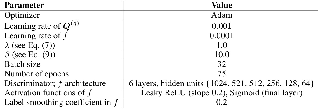
🔼 This table lists the hyperparameters used in the domain adaptation experiments. It includes the optimizer used (Adam), learning rates for the Q matrices, the discriminator f, and the classifier, the batch size, number of epochs, the discriminator’s architecture (6-layer MLP with specified hidden units), activation functions (Leaky ReLU and sigmoid), and a label smoothing coefficient.
read the caption
Table 7: Hyperparameter settings for domain adaptation.

🔼 This table presents the classification accuracy results for the Office-31 dataset’s domain adaptation task using ResNet50 embeddings. It compares the performance of the proposed method against several baselines (DANN, MDD, MCC, SDAT, ELS) across different source-target domain combinations (A-W, D-W, W-D, A-D, D-A, W-A). The accuracy is presented as mean ± standard deviation, highlighting the performance variability and offering a comprehensive comparison of the proposed approach against established domain adaptation techniques.
read the caption
Table 1: Classification accuracy on the target domain of office-31 dataset (ResNet50 embedding).
🔼 This table presents the classification accuracy results on the target domain (Office-31 dataset) using ResNet50 embeddings as features. It compares the performance of the proposed method against several state-of-the-art domain adaptation techniques (DANN, MDD, MCC, SDAT, ELS). The results are shown for different source-target domain combinations (e.g., A-W represents Amazon to Webcam). The table demonstrates that the proposed approach achieves higher accuracy in most of the domain adaptation tasks compared to existing methods.
read the caption
Table 1: Classification accuracy on the target domain of office-31 dataset (ResNet50 embedding).
Full paper#


