↗ OpenReview ↗ NeurIPS Homepage ↗ Chat
TL;DR#
Current recurrent solvers struggle with reasoning tasks, especially when input dimensionality increases. They often fail to maintain performance on harder versions of a task and cannot handle problems where input and output sizes differ. This paper tackles these limitations.
NeuralSolver, a novel recurrent solver with three components—a recurrent module, a processing module, and a curriculum-based training scheme—addresses these issues. It consistently outperforms state-of-the-art methods in extrapolation, handles various problem sizes, and achieves higher efficiency in training and parameters.
Key Takeaways#
Why does it matter?#
This paper is important because it introduces NeuralSolver, a novel recurrent solver that surpasses existing methods in consistent and efficient extrapolation across diverse tasks. Its ability to handle both same-size and different-size problems opens new avenues for research in algorithm learning and reasoning. The novel different-size tasks presented also advance the field. The efficiency gains, requiring 90% fewer parameters, are significant for resource-constrained applications.
Visual Insights#

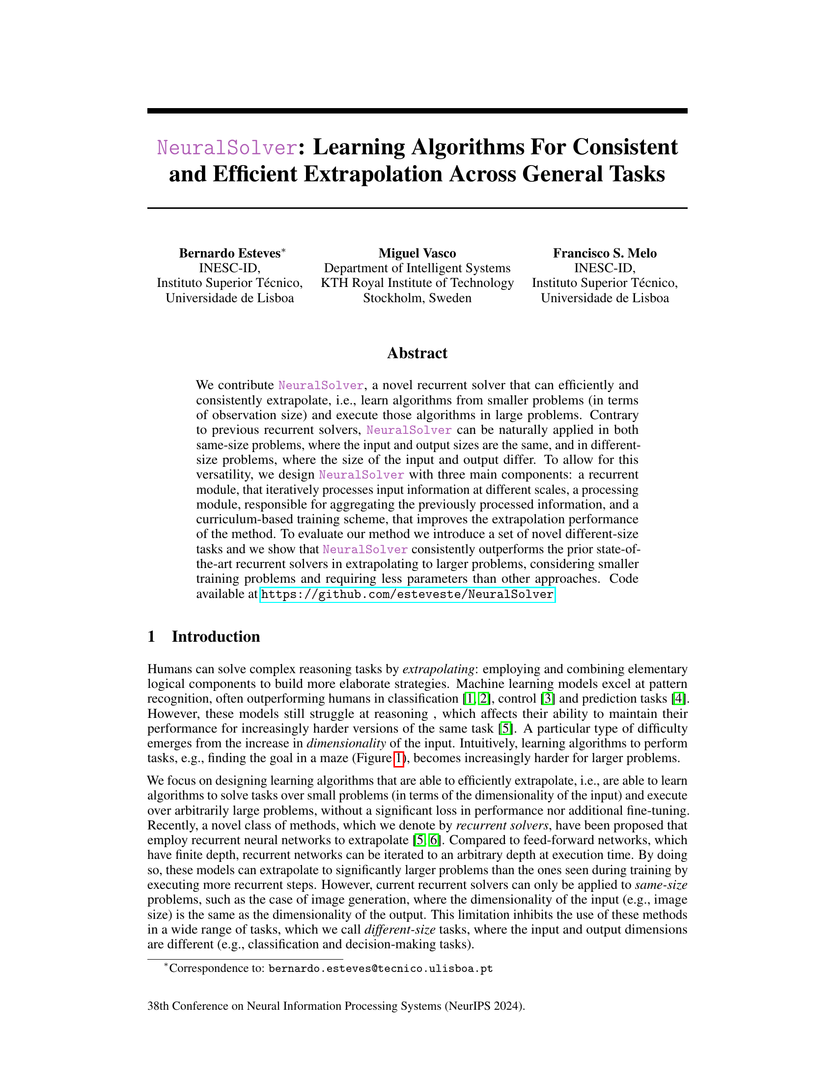
This figure shows four different sizes of the 1S-Maze environment. The green square represents the agent, and the red square represents the goal. The agent must navigate the maze to reach the goal. The light green arrow indicates the next action the agent should take, and the purple path shows the optimal solution path.

This table compares the extrapolation accuracy of NeuralSolver against several baseline models on same-size tasks. The tasks include Prefix-Sum, Maze, Thin-Maze, and Chess, each with varying training and testing sizes. The results show NeuralSolver’s superior performance in extrapolating to larger problems, particularly when compared to Bansal et al. [6], both with and without progressive loss.
In-depth insights#
NeuralSolver Design#
The NeuralSolver architecture is thoughtfully designed for consistent and efficient extrapolation. It leverages a recurrent convolutional module to process input data at multiple scales, enabling it to handle varying input sizes effectively. This recurrent module’s iterative processing allows for extrapolation beyond the training data’s dimensionality. A key innovation is the inclusion of a processing module, responsible for aggregating the processed information and generating the output. This module allows NeuralSolver to seamlessly handle both same-size and different-size tasks, a significant improvement over existing recurrent solvers. Finally, a curriculum-based training scheme enhances the model’s extrapolation capabilities by gradually increasing the input size during training, thus improving its ability to generalize to larger, unseen problems. This layered approach, combining recurrent processing with adaptable aggregation and curriculum learning, positions NeuralSolver as a robust and versatile algorithm solver.
Extrapolation Tasks#
The concept of “Extrapolation Tasks” in a research paper likely refers to the methods used to evaluate a model’s ability to generalize beyond its training data. This is crucial for assessing the true capabilities of a model, as a model that only performs well on its training data is not truly robust or intelligent. These tasks would involve presenting the model with significantly larger or more complex problems than those it was trained on. The success or failure on these extrapolation tasks would then highlight the model’s ability to learn underlying principles rather than simply memorizing patterns, a key factor in determining the model’s generalizability and real-world applicability. Careful selection of these tasks is critical to ensure they accurately reflect the type of extrapolation needed for the problem at hand and avoid biases in the evaluation process. The paper likely details the design, implementation, and results of these extrapolation tasks, providing valuable insight into the model’s strengths and weaknesses in handling unseen scenarios.
Curriculum Learning#
Curriculum learning, in the context of the NeuralSolver paper, is a crucial training strategy that gradually increases the complexity of training tasks. It starts with simpler, smaller-sized problems and progresses to larger, more complex ones. This approach is particularly relevant because NeuralSolver is designed to extrapolate learned algorithms to problems significantly larger than those seen during training. The paper highlights the importance of curriculum learning in improving extrapolation performance, suggesting that it mitigates challenges like a reduced training signal in different-size tasks where the output dimensionality is smaller than the input. By using a curriculum-based training scheme, NeuralSolver can learn effective algorithms from relatively small problems and then robustly generalize them to much larger problems. The method employs a strategy of gradually increasing the dimensionality of the observations in different-size tasks, helping prevent catastrophic forgetting and boosting the ability to handle increasingly larger inputs. The effectiveness of this approach is empirically demonstrated in the experiments, where NeuralSolver outperforms previous methods in both same-size and different-size tasks.
Ablation Experiments#
Ablation experiments systematically remove components of a model to assess their individual contributions. In this context, it would involve removing parts of the NeuralSolver architecture (recurrent module, processing module, curriculum learning) one at a time to understand how each impacts performance. The key insight sought is to determine which aspects are crucial for consistent and efficient extrapolation. Results would likely show that all three components contribute significantly, with the recurrent module and its ability to process varying scales of input being particularly critical for handling the different-size tasks. Curriculum learning’s impact might be less dramatic, suggesting the model’s architecture itself is a stronger driver of extrapolation ability than the training regime. The ablation study helps isolate the core strengths of the NeuralSolver and highlights design choices that would be important to retain for future improvements or adaptations.
Future Work#
The paper’s conclusion mentions future work focusing on improving training efficiency and exploring reinforcement learning applications. Specifically, they aim to enhance NeuralSolver’s ability to learn algorithms from fewer examples while maintaining its extrapolation capabilities. Applying it to online, sequential decision-making tasks is another key goal, potentially impacting fields requiring real-time adaptability. Extending the model to handle more complex scenarios and evaluating its performance on diverse tasks would further demonstrate its robustness and versatility. Addressing the challenges related to generalization across various tasks and environments is critical for broader applicability. The exploration of different architectural modifications and hyperparameter optimization to enhance performance is also warranted. Overall, future research will likely focus on expanding NeuralSolver’s capabilities and solidifying its position within the broader field of AI.
More visual insights#
More on figures

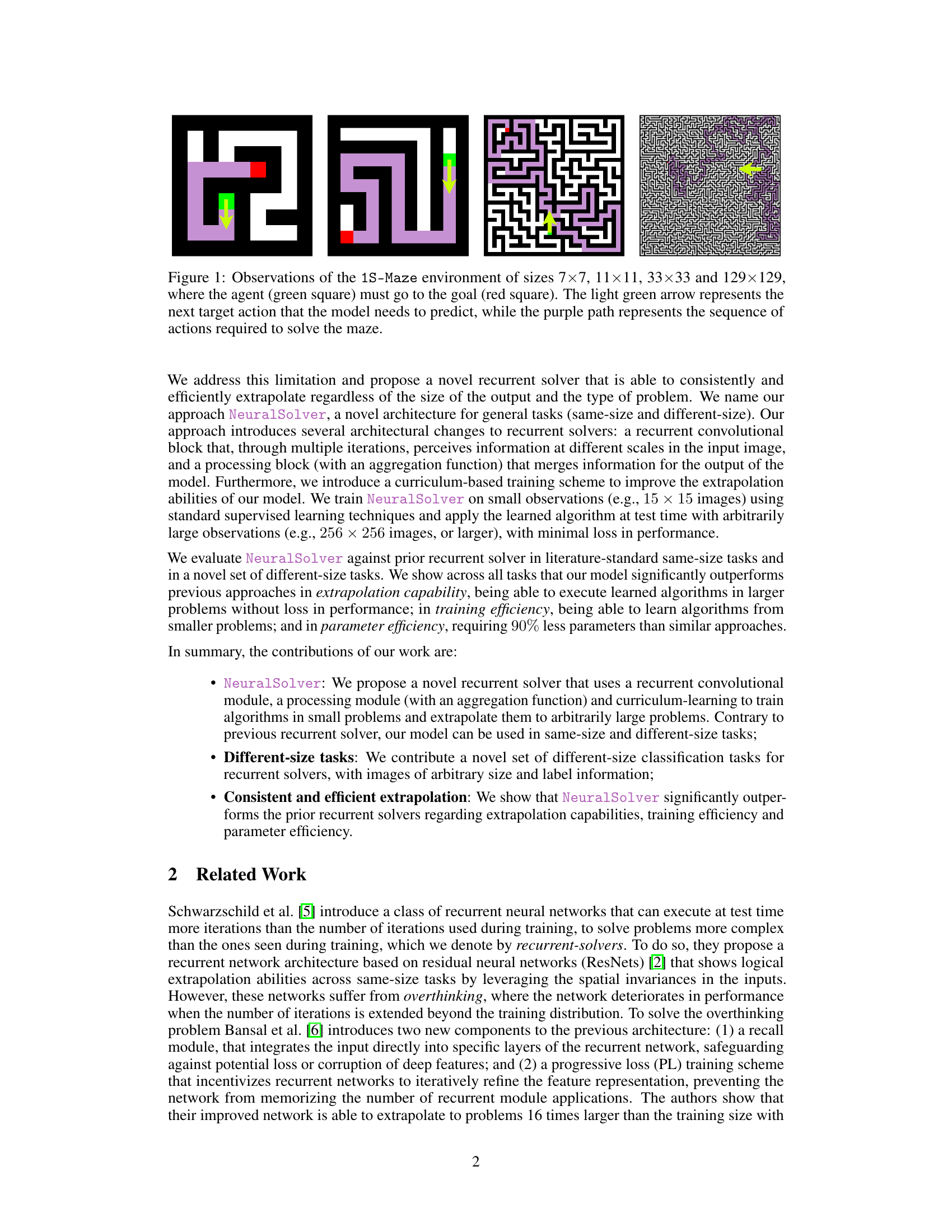
This figure illustrates the architecture of NeuralSolver, highlighting its two main components: a recurrent module for iterative data processing and a processing module for output generation. The recurrent module handles inputs of varying sizes, while the processing module (with optional aggregation) allows for both same-size and different-size tasks. A curriculum-based training scheme enhances extrapolation.

The figure visualizes how information propagates through NeuralSolver’s recurrent module during maze solving. The top row shows the difference between the internal state at each iteration and the final state, indicating convergence. The bottom row displays the action probabilities at each iteration, illustrating how the model’s certainty about the next action increases as the internal state converges.

This figure shows four different classification tasks used to evaluate the NeuralSolver model. Each task involves an image input of arbitrary size, representing different game-like scenarios (GoTo, 1S-Maze, Pong, DoorKey). The model must predict a one-hot encoded vector indicating the appropriate action. The number of possible actions varies across the tasks (4, 4, 3, and 4 respectively). These tasks test the NeuralSolver’s ability to extrapolate to different sizes.

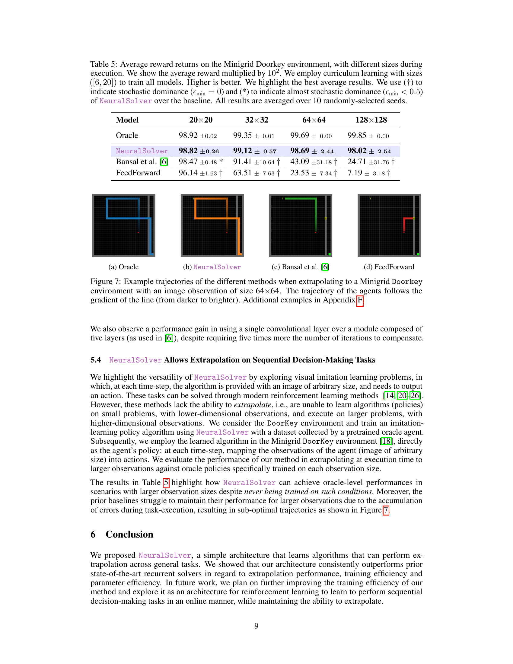
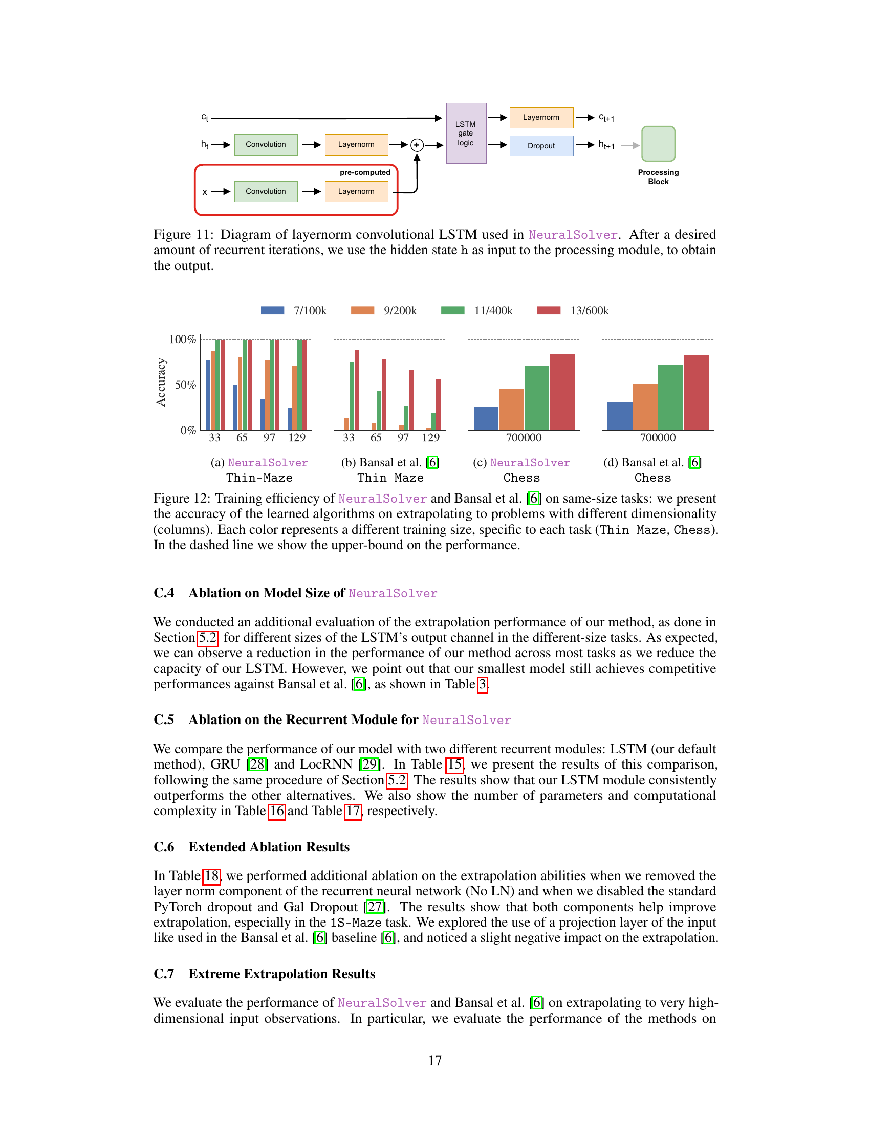
This figure compares the training efficiency of NeuralSolver and Bansal et al.’s model on same-size tasks. It shows the accuracy of learned algorithms when extrapolating to problems of varying sizes, with different training sizes represented by different colors. The dashed line indicates the upper bound on performance.

The figure shows the performance of NeuralSolver and Bansal et al. [6] on same-size tasks, demonstrating training efficiency. It displays the accuracy of learned algorithms when extrapolating to problems of varying dimensionality (different problem sizes). Each color represents a different training size for each task, with details in Appendix A.3. A dashed line indicates the upper performance bound.

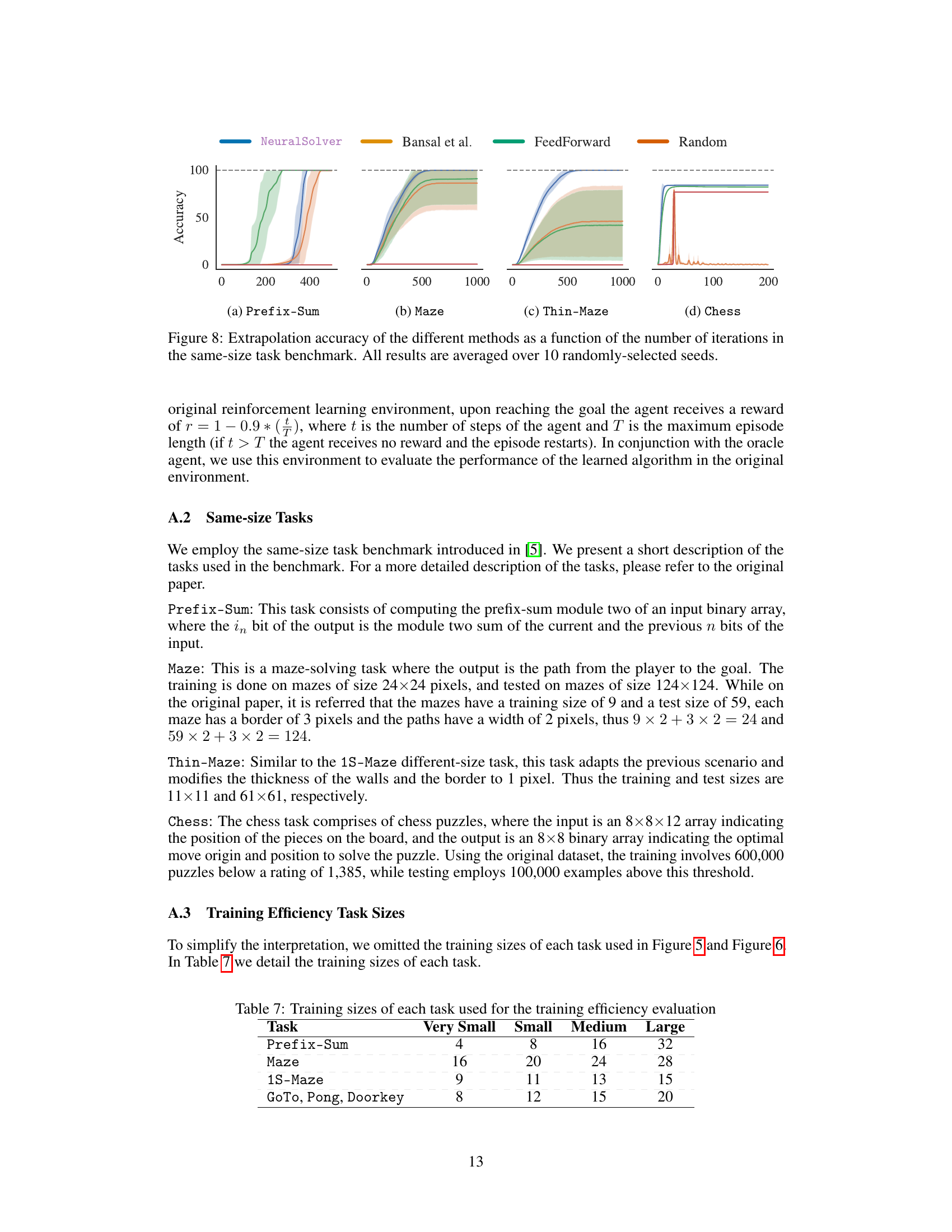
This figure compares the extrapolation accuracy of four different models (NeuralSolver, Bansal et al., FeedForward, and Random) across four different same-size tasks (Prefix-Sum, Maze, Thin-Maze, and Chess). The x-axis represents the number of iterations performed, and the y-axis represents the accuracy achieved. The shaded regions represent the standard deviations across 10 different runs. This figure demonstrates the extrapolation capabilities of each model by showing how accuracy increases (or decreases) with more iterations, showcasing the performance gains of NeuralSolver over the other models.

This figure compares the training efficiency of NeuralSolver and Bansal et al.’s model on same-size tasks. It shows how well each model extrapolates to problems of different sizes after being trained on smaller datasets. Each color represents a different training set size for each task. The dashed line indicates the upper-bound performance, showcasing the optimal performance possible.

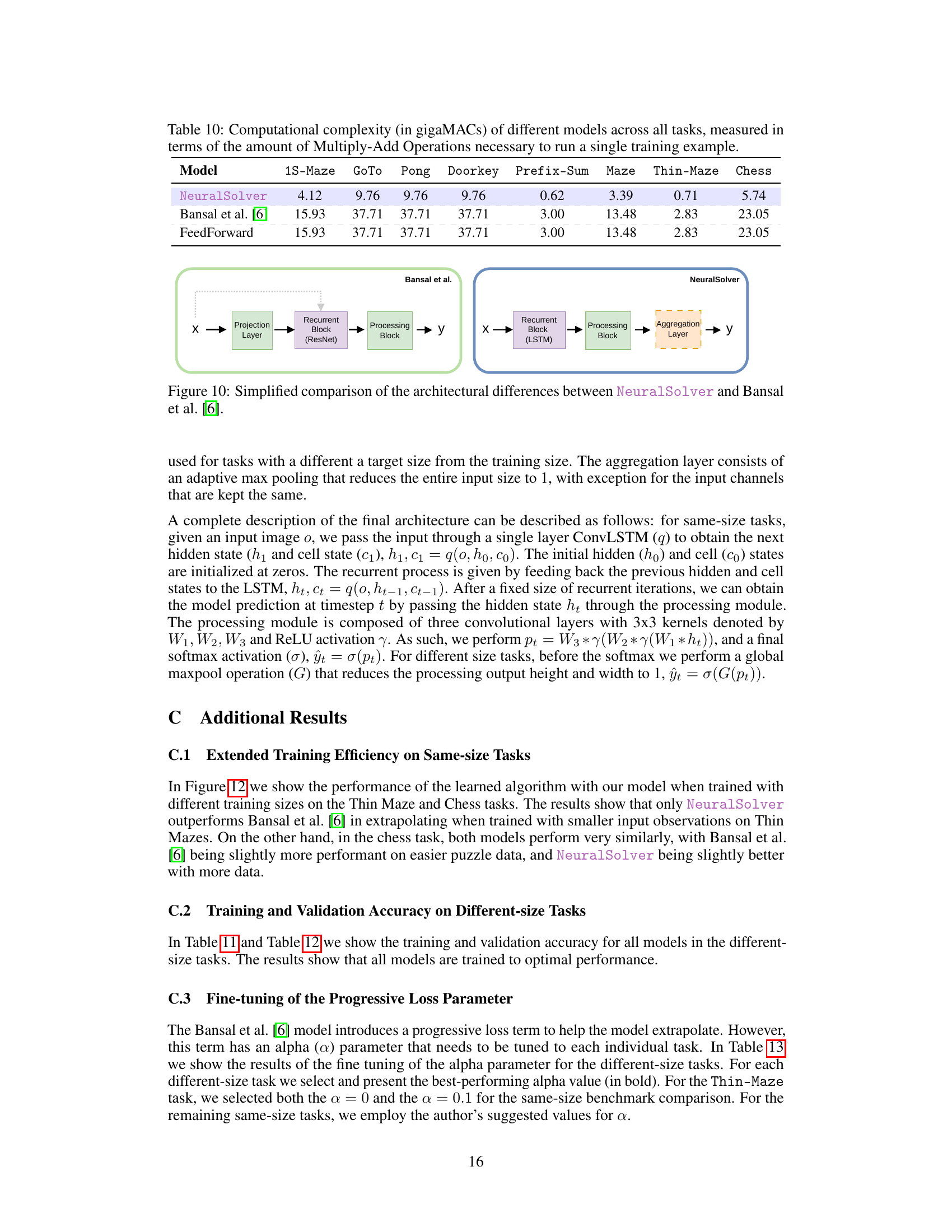
The figure shows a simplified comparison of the architectures of NeuralSolver and the Bansal et al. recurrent solver. NeuralSolver removes the projection layer present in Bansal et al. and replaces the ResNet recurrent block with a convolutional LSTM. A key difference is the addition of an aggregation layer in NeuralSolver’s processing module, enabling it to handle both same-size and different-size tasks.

This figure shows the architecture of the layernorm convolutional LSTM used in the NeuralSolver model. The diagram details the flow of information through the LSTM cell, including the input (x), hidden state (ht), cell state (ct), convolutional and layernorm layers, and dropout layer. The pre-computed convolutional and layernorm layers are highlighted to show computational efficiency. The output (ht+1) of the recurrent module is then passed to the processing block for final output generation.

This figure compares the training efficiency of NeuralSolver and Bansal et al.’s model on same-size tasks. It shows how the accuracy of learned algorithms changes when extrapolating to problems of different dimensionalities, using different training sizes for each task. The dashed line represents the upper bound of performance.
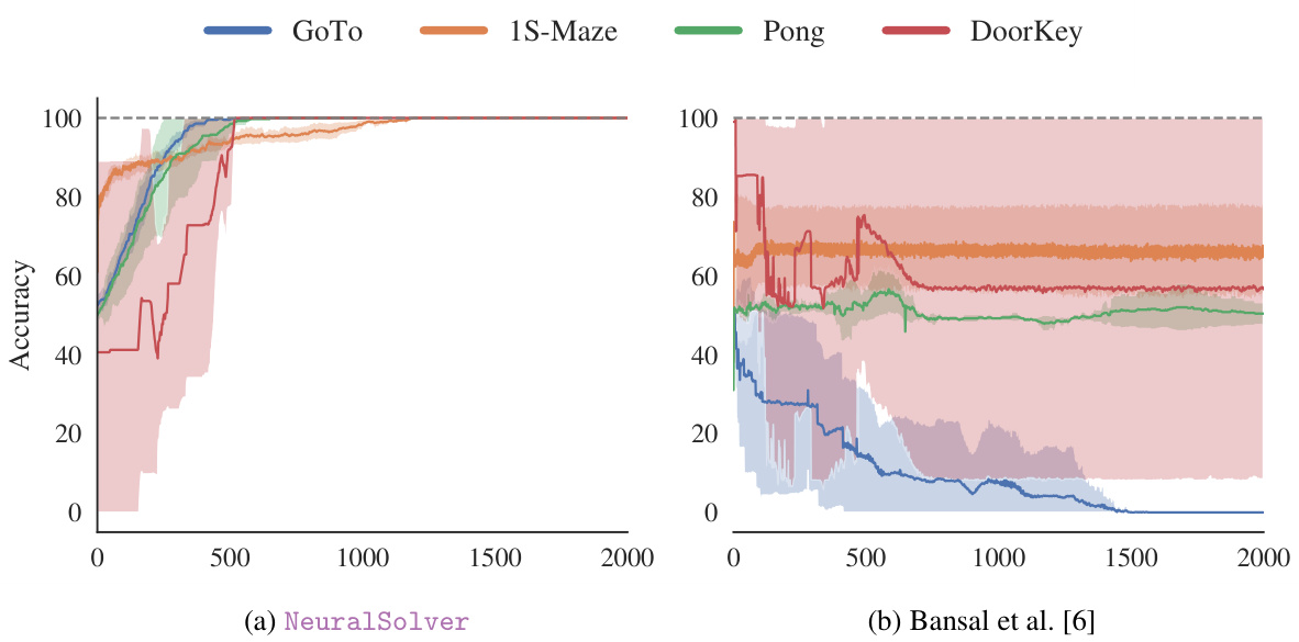
The figure shows the accuracy of NeuralSolver and Bansal et al. [6] on same-size tasks when trained with different training sizes. The x-axis represents the size of the problem being tested, and the y-axis represents the accuracy achieved. Different colors correspond to models trained on problems of different sizes. The dashed line indicates the upper bound of performance achievable on each task. This illustrates the training efficiency of each model; NeuralSolver is more efficient in training and extrapolating to larger problems than Bansal et al. [6].
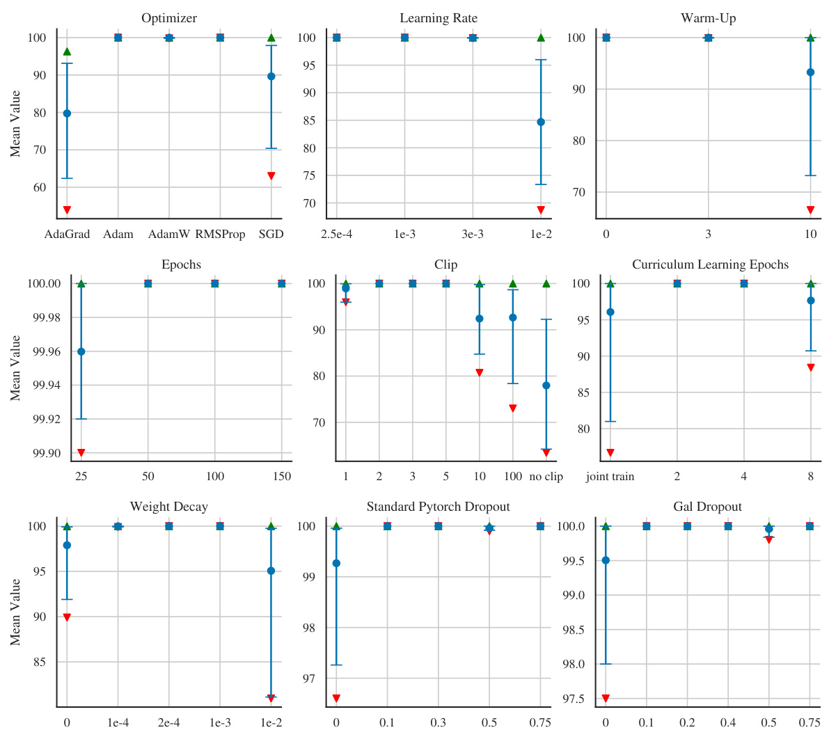
This figure shows the results of a hyperparameter search for the NeuralSolver model on the GoTo task. Each subplot shows the effect of varying a single hyperparameter (optimizer, learning rate, warm-up, epochs, clip value, curriculum learning epochs, weight decay, standard PyTorch dropout, and Gal dropout) while holding others constant at the values specified in Table 9 of the paper. The mean performance is shown with error bars representing 95% confidence intervals. The green and red arrows indicate the maximum and minimum values observed during bootstrapping, providing insight into the range of performance.
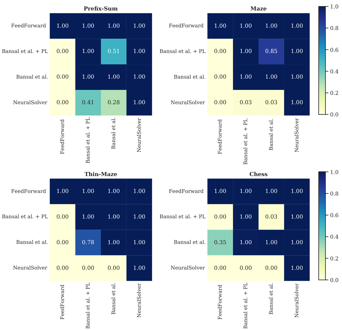
This figure shows the results of the Almost Stochastic Order (ASO) test comparing different recurrent solvers on same-size tasks. The ASO test determines statistical significance by measuring the stochastic dominance of one model over another. The color intensity represents the emin value, indicating how much one model outperforms another. Darker colors mean more significant dominance. For instance, NeuralSolver is shown to significantly outperform Bansal et al. in most cases.

This figure shows the results of the Almost Stochastic Order (ASO) test comparing the performance of NeuralSolver against the baselines on the different-size tasks. The ASO test determines the statistical significance of the performance difference between two models. A lower min score indicates that the model in the row is stochastically dominant over the model in the column. The results demonstrate NeuralSolver’s significant performance improvement compared to the baselines across all tasks.
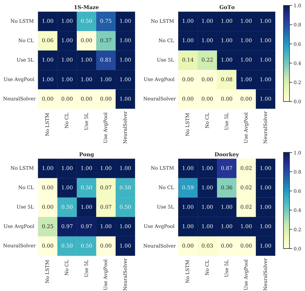
This figure shows the results of an ablation study on different components of the NeuralSolver model for different-size tasks. The Almost Stochastic Order (ASO) test is used to compare the performance of different model variants. The heatmap visually represents the statistical significance of performance differences. For example, NeuralSolver is significantly better than the model without LSTMs in the 1S-Maze task.

This figure shows examples of the 1S-Maze environment with different sizes (7x7, 11x11, 33x33, and 129x129). Each image shows the agent (green square), the goal (red square), the next action the agent should take (light green arrow), and the optimal path to the goal (purple line). The figure illustrates the increasing complexity of the task with larger maze sizes.

This figure shows the results of the Almost Stochastic Order (ASO) test performed on the different-size tasks. The ASO test compares the performance of different algorithms by considering their scores across multiple runs. The results are presented as a heatmap, with each cell representing the minimum value (∈min) of the ASO test comparing two algorithms. A value of ∈min < 0.5 indicates almost stochastic dominance, while ∈min = 0.0 indicates stochastic dominance. The heatmap helps visualize which algorithm performs statistically significantly better than others for each task.

This figure visualizes how information propagates through NeuralSolver’s recurrent module during maze solving. The top row shows the difference between the internal state at each iteration and the final state, highlighting convergence. Darker blue indicates larger differences. The bottom shows action probabilities at each iteration, demonstrating how the model’s certainty increases as the recurrent module converges.

This figure visualizes how information propagates through the NeuralSolver’s recurrent module when solving the 1S-Maze task. The top row shows the difference between the internal state at each iteration and the final state, highlighting areas that have converged. Darker blue indicates larger differences. The bottom row displays the model’s predicted action probabilities (R, D, L, U) at each iteration.

This figure shows how information propagates through the NeuralSolver model during maze solving. The top row displays the differences between the internal state at each iteration and the final state, visualizing the convergence of the model’s internal representation. Darker blue indicates larger differences, showing which parts of the maze are still being processed. The bottom row presents the action probabilities predicted by the model at different iteration steps, illustrating how the model’s understanding of the optimal path evolves over time.

The figure shows how information propagates through the NeuralSolver model’s recurrent module during the execution of a maze-solving task. The top row visualizes the differences between the internal state at each iteration and the final state, highlighting how the model focuses on certain areas as it progresses through the iterations. The bottom row shows the model’s prediction of the agent’s next action (R, D, L, or U) at each iteration, illustrating how the uncertainty of the prediction decreases as the recurrent module’s state converges towards the final solution.

This figure visualizes how information propagates through the NeuralSolver model during the maze-solving process. The top row shows the difference in internal state values between each iteration and the final iteration; larger differences are depicted in darker blue, while smaller differences are in white. This illustrates how the model’s internal representation of the maze evolves with each step. The bottom row displays the action probabilities predicted by the model’s processing module at different iterations. The arrows (R, D, L, U) represent the agent’s possible actions: right, down, left, and up.
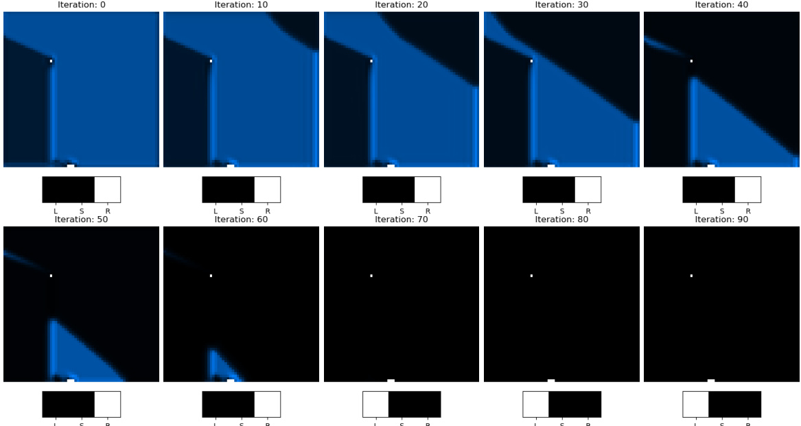
This figure visualizes how information propagates through the NeuralSolver model during the execution of a maze-solving task. The top row shows the difference between the internal state of the recurrent module at each iteration and its final state. Darker blue indicates larger differences, meaning that those parts of the maze are still being processed. The bottom row displays the action probabilities at each iteration. It shows how the model’s certainty about the next action increases as the number of iterations increases and the internal state converges to the solution.

This figure visualizes how information propagates through the NeuralSolver model while solving a 1S-Maze task. The top row shows the differences between the internal state at each iteration and the final state, with white pixels indicating convergence. The bottom row displays the action probabilities predicted by the model at different iterations.
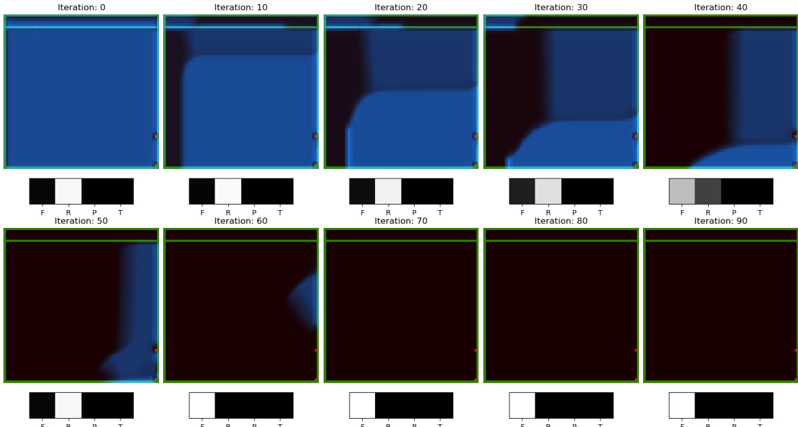
This figure visualizes how information propagates through the neural network’s recurrent module during the DoorKey task. The top row shows the difference in the internal state between consecutive iterations, with white representing convergence to a stable state and dark blue showing large differences. The bottom row shows the model’s predicted probabilities for different actions (Forward, Rotate Right, Pickup, Toggle) at each iteration. It illustrates the network’s learning process by showing how its internal representation evolves and leads to the correct action prediction.

This figure shows how information propagates through the network when solving the Doorkey task. The top row shows the difference between the internal state at the current iteration and the last iteration. The bottom row shows the predicted action probabilities. The figure demonstrates how NeuralSolver solves the task by iteratively processing information and converging to a solution.

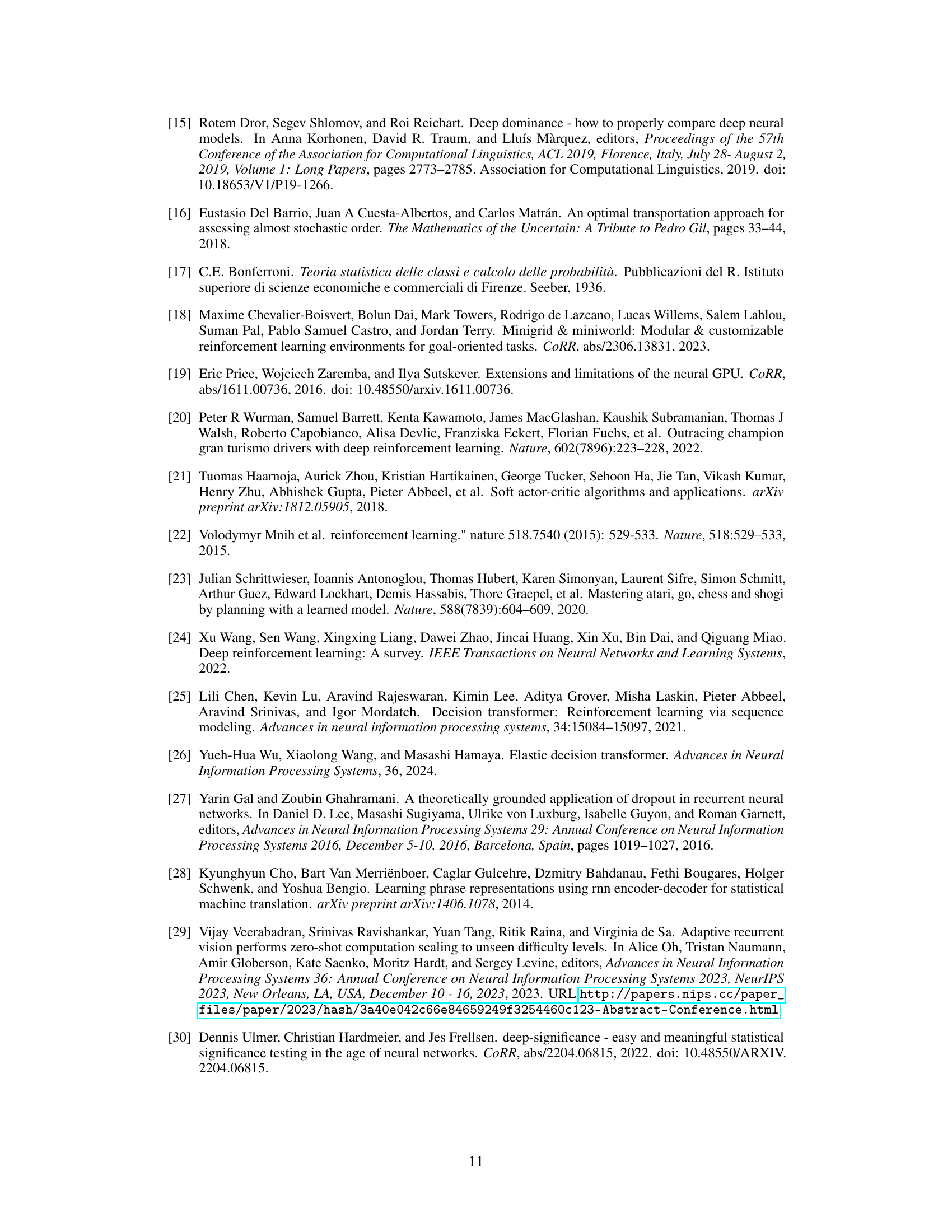
This figure visualizes the trajectories of four different models (Oracle, NeuralSolver, Bansal et al., and FeedForward) in a Minigrid Doorkey environment with varying sizes (32x32, 64x64, and 128x128). Each row shows a different task, illustrating how well each model performs compared to the optimal Oracle trajectory in navigating the environment.

This figure shows an example of a 1S-Maze task used in the paper’s experiments. The image is significantly larger than those used during training (512 x 512 pixels), demonstrating the model’s ability to extrapolate to larger problem sizes. The maze is complex and the path to the goal is not immediately obvious, highlighting the challenge addressed by the NeuralSolver model.

This figure shows how information propagates through the NeuralSolver model during maze solving. The top panel displays the difference between the internal state at each iteration and the final state, visualizing the convergence of the model. Darker blue indicates larger differences. The bottom panel shows the action probabilities predicted at each step, demonstrating the decision-making process of the model.
More on tables

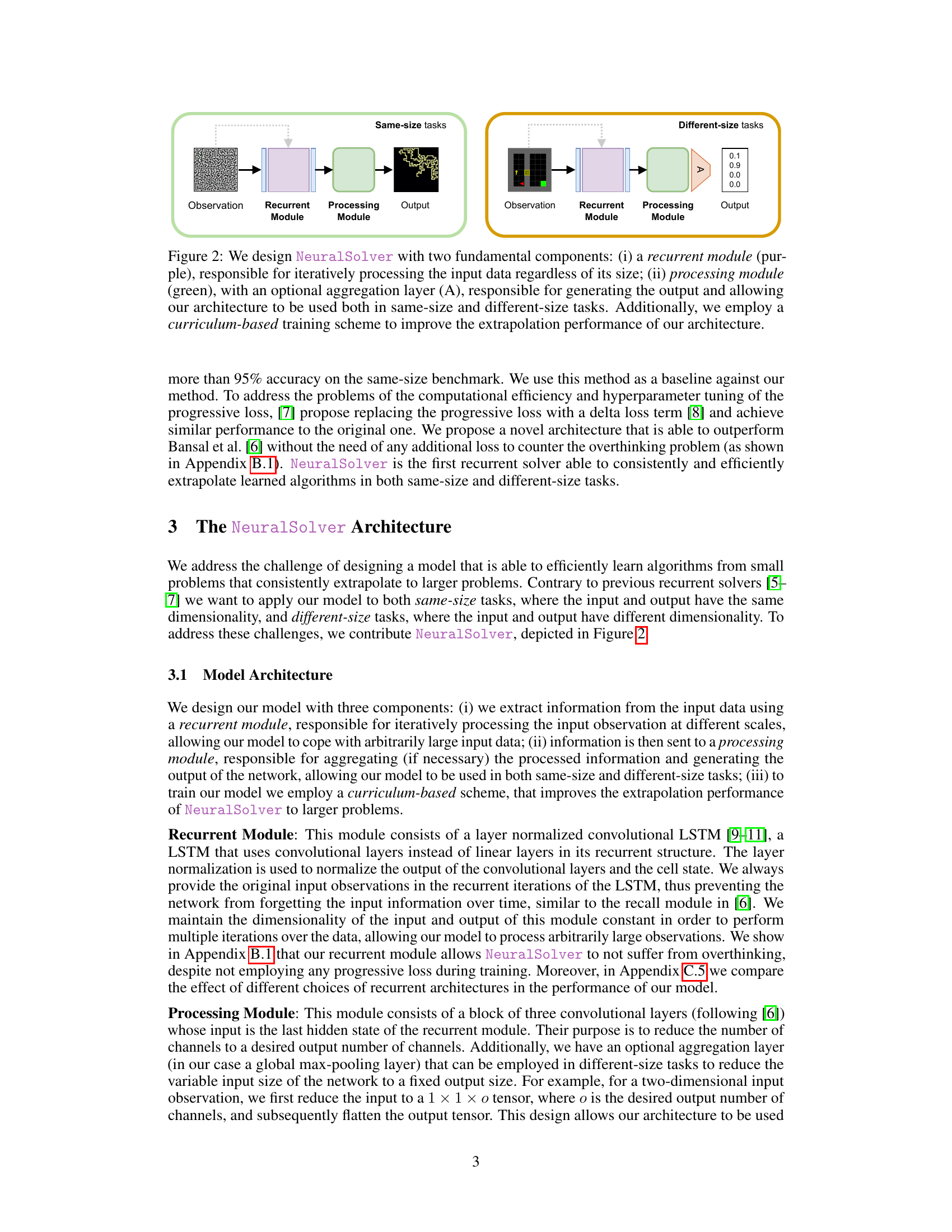
This table presents the total number of parameters (in millions) for different models evaluated on same-size tasks (Prefix-Sum, Maze, Thin-Maze, Chess). It shows the parameter efficiency of NeuralSolver compared to the baselines (Bansal et al. [6] and FeedForward). NeuralSolver demonstrates significantly fewer parameters.

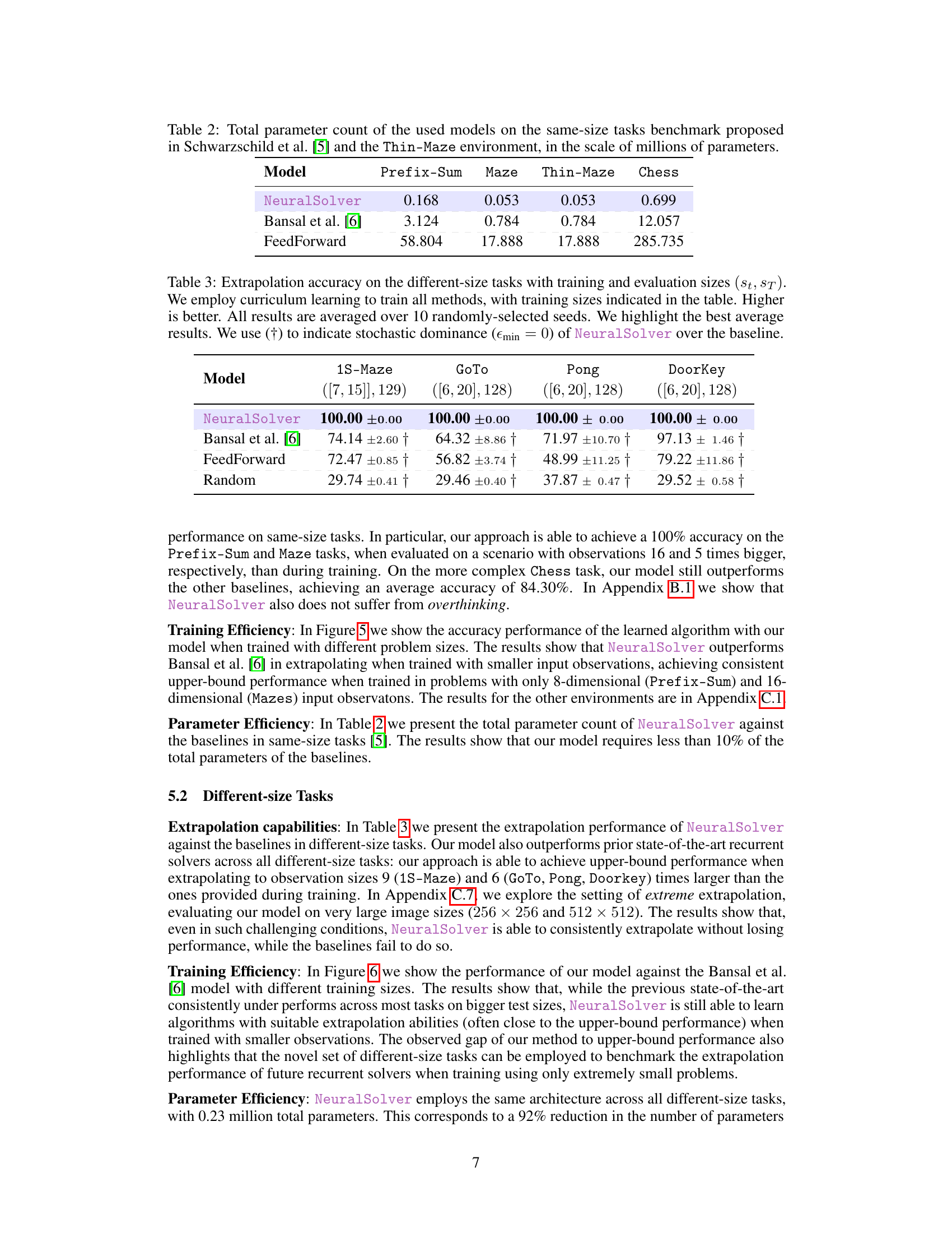
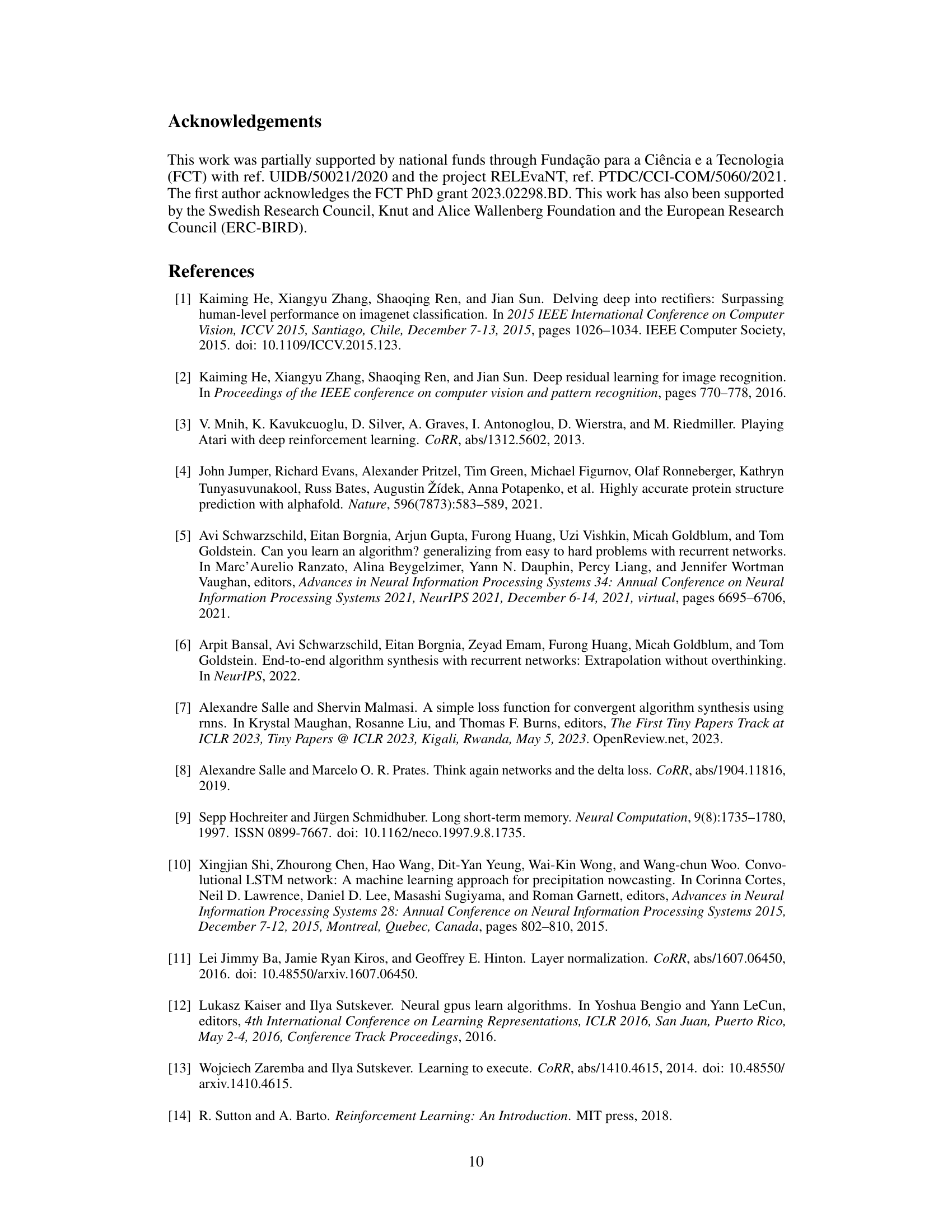
This table presents the extrapolation accuracy results for four different-size tasks (1S-Maze, GoTo, Pong, DoorKey). The results compare the performance of NeuralSolver against three baseline methods: Bansal et al. [6], FeedForward, and Random. Curriculum learning was used in training. The table highlights the best average results across ten random seeds and uses the † symbol to indicate when NeuralSolver shows stochastic dominance over the baselines.

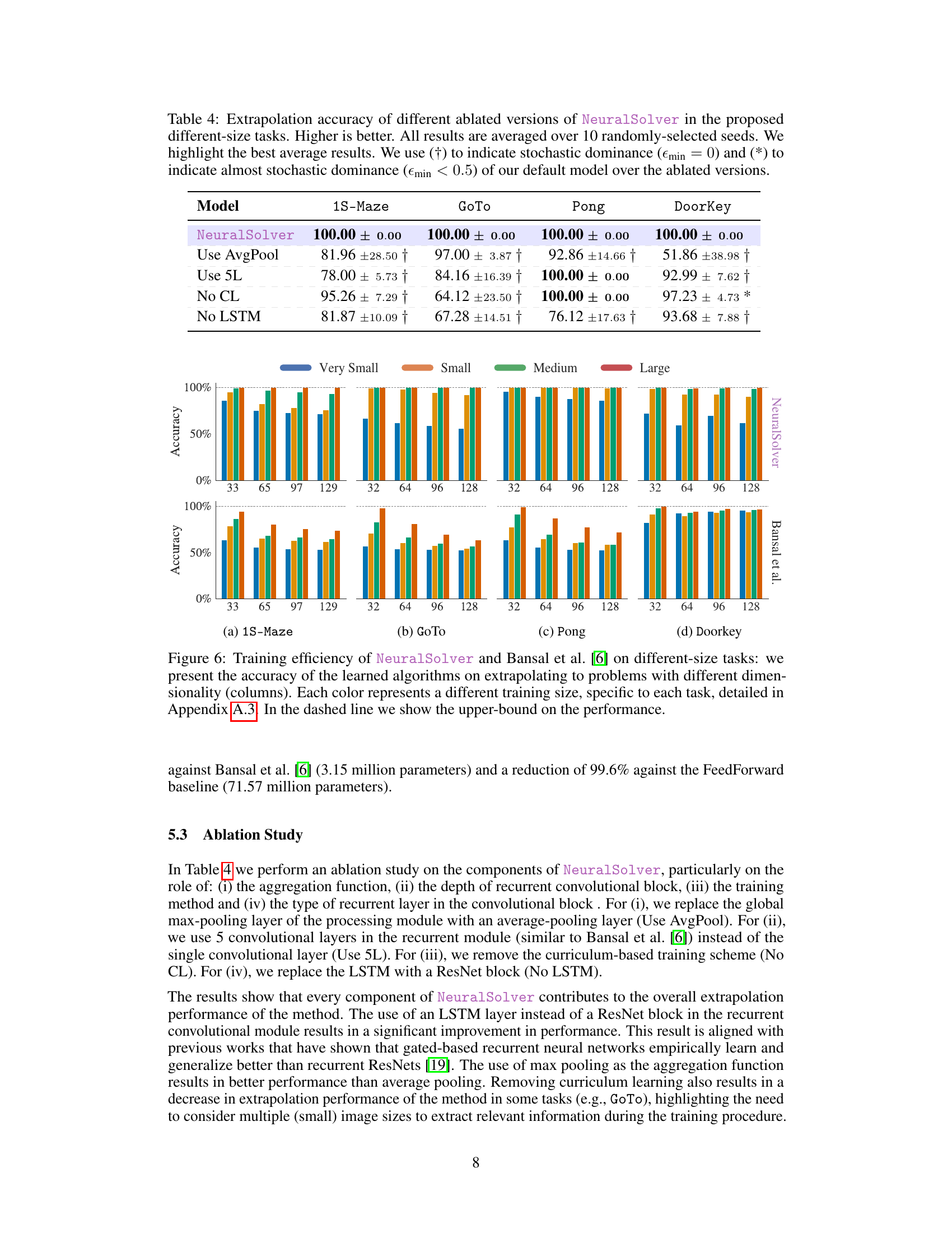
This table presents the ablation study on the NeuralSolver model by removing different components of the model to demonstrate how each component contributes to the overall performance. It shows the extrapolation accuracy on four different-size tasks (1S-Maze, GoTo, Pong, DoorKey) for the following variations: - NeuralSolver: The complete model. - Use AvgPool: Replaced the global max-pooling layer with an average-pooling layer. - Use 5L: Used 5 convolutional layers in the recurrent module instead of 1. - No CL: Removed the curriculum-based training scheme. - No LSTM: Replaced the LSTM with a ResNet block. The results demonstrate the impact of each component on the model’s ability to extrapolate.
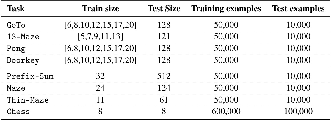
This table shows the training and test sizes for each task used in the paper’s experiments. It also details the number of training and test examples for each task. For the different-size tasks, which involve a curriculum-based training scheme, the table specifies the dimensions of training examples at different stages of the curriculum.

This table compares the extrapolation accuracy of NeuralSolver against baselines (Bansal et al. [6] with and without progressive loss, and a feedforward network) on same-size tasks. It shows the accuracy achieved on four tasks (Prefix-Sum, Maze, Thin-Maze, and Chess) with different training and evaluation sizes. The results highlight NeuralSolver’s superior performance, particularly in extrapolating to larger problems.

This table shows the extrapolation accuracy of NeuralSolver and other baseline models on same-size tasks. It compares the performance of NeuralSolver against Bansal et al. [6] with and without progressive loss, as well as a feedforward network. The results are averaged over 10 random seeds, and statistical significance is indicated. The table demonstrates NeuralSolver’s superior extrapolation capabilities by highlighting the best average results and noting where it stochastically dominates the baselines.

This table presents the extrapolation accuracy results of NeuralSolver and three baseline models (Bansal et al. [6] with and without progressive loss, and a feedforward network) on four same-size tasks (Prefix-Sum, Maze, Thin-Maze, Chess). It shows the accuracy achieved when the model is trained on smaller problem sizes and then tested on larger problem sizes (extrapolation). The table highlights the superior performance of NeuralSolver in consistently achieving near-perfect accuracy even when extrapolating to significantly larger problem sizes than those seen during training. Stochastic dominance is used to statistically compare NeuralSolver against the baselines, demonstrating its superiority.

This table presents the computational complexity, measured in Giga Millions of Multiply-Accumulate operations (GMACs), for different models across various tasks. It compares NeuralSolver against the Bansal et al. [6] and FeedForward models. Lower GMACs indicate greater computational efficiency.

This table shows the extrapolation accuracy of NeuralSolver and baseline models on four different-size tasks. It highlights the best performance for each task and indicates when NeuralSolver stochastically dominates the baseline models. Curriculum learning was used in training, and training sizes are specified.

This table presents the extrapolation accuracy results for different-size tasks. It compares the performance of NeuralSolver against baselines (Bansal et al. [6], FeedForward, Random). The table shows accuracy with standard deviations, highlights the best-performing model for each task, and uses a symbol (†) to indicate when NeuralSolver stochastically dominates a baseline.

This table presents the extrapolation accuracy achieved by the NeuralSolver model across five different-size tasks (1S-Maze, GoTo, Pong, DoorKey, Thin-Maze) for various values of the alpha (α) parameter used in the progressive loss training scheme. Each row represents a different α value, and each column shows the average accuracy and standard deviation for a specific task. The results highlight how the choice of α impacts the model’s ability to extrapolate across tasks of varying size and complexity.

This table presents the results of an ablation study conducted to evaluate the impact of varying the number of channels in the LSTM’s output and hidden state (model width) on the extrapolation performance of the NeuralSolver model across four different-size tasks. The table shows that a model width of 64 (the default setting) achieves the best performance overall. Reducing the model width leads to a decrease in performance, particularly in the 1S-Maze and DoorKey tasks.

This table presents the extrapolation accuracy results achieved by the NeuralSolver model using three different recurrent modules: LSTM (the default module used in the paper), GRU, and LocRNN. The results are shown for four different-size tasks (1S-Maze, GoTo, Pong, and Doorkey). The table highlights the performance of each recurrent module in terms of accuracy and helps determine the optimal recurrent module for the NeuralSolver model in different-size tasks.

This table presents a comparison of the total number of parameters (in millions) for the NeuralSolver model when using different recurrent modules (LSTM, GRU, LocRNN) across four different-size tasks. The goal is to show the parameter efficiency of NeuralSolver, with lower numbers indicating better performance. The default model uses an LSTM.

This table presents the total number of parameters (in millions) used by the NeuralSolver model with different recurrent modules (LSTM, GRU, LocRNN) across different tasks. A lower number of parameters indicates higher parameter efficiency. The table highlights the parameter efficiency of the NeuralSolver model, especially when compared to other models discussed in the paper.

This table presents the ablation study of the NeuralSolver model. It shows the extrapolation accuracy of different versions of the model where some components are removed or replaced to analyze their impact on the overall performance. The results show the performance of different-size tasks with different components removed or replaced. The comparison is done against the default model using Almost Stochastic Dominance test. The table highlights the best performing model for each task and identifies which alterations resulted in a statistically significant drop in performance.

This table presents the extrapolation accuracy of NeuralSolver and baseline models on four different-size tasks. Curriculum learning was used during training. The results show NeuralSolver’s superior performance in extrapolation, consistently achieving higher accuracy compared to the baselines across different tasks and larger problem sizes.

This table presents the extrapolation accuracy of NeuralSolver and baseline models on four different-size tasks. It shows the performance of each model when trained on smaller datasets and tested on larger datasets, highlighting the model’s ability to extrapolate. The results are averaged over ten runs, and statistical significance is assessed using the Almost Stochastic Order (ASO) test.
Full paper#
