↗ OpenReview ↗ NeurIPS Homepage ↗ Hugging Face ↗ Chat
TL;DR#
Solving partial differential equations (PDEs) is computationally expensive, especially for complex problems. Traditional numerical methods often struggle with sample efficiency and generalization to unseen data. Machine learning offers potential solutions but existing operator learning methods also face limitations like requiring massive datasets for effective training.
The paper introduces POSEIDON, a foundation model addressing these issues. It uses a multiscale operator transformer with a novel training strategy to significantly improve sample efficiency and accuracy. POSEIDON’s success is demonstrated on diverse downstream tasks, showcasing its generalizability to a wide range of PDE types. The availability of open-source code and datasets further advances its potential usage in PDE-related research.
Key Takeaways#
Why does it matter?#
This paper is crucial for researchers in the fields of scientific machine learning and partial differential equations because it introduces a novel foundation model, POSEIDON, that significantly improves upon existing methods in terms of sample efficiency and accuracy. Its ability to generalize to unseen PDEs opens new avenues for research and applications. The open-sourcing of the model and datasets further enhances its impact on the broader research community.
Visual Insights#

The figure compares the sample efficiency of POSEIDON, a pretrained foundation model for PDEs, against task-specific neural operators. It shows that POSEIDON requires significantly fewer training samples to achieve similar accuracy compared to task-specific models. Additionally, POSEIDON demonstrates the ability to generalize to unseen physics during finetuning, showcasing its potential as a general-purpose model.
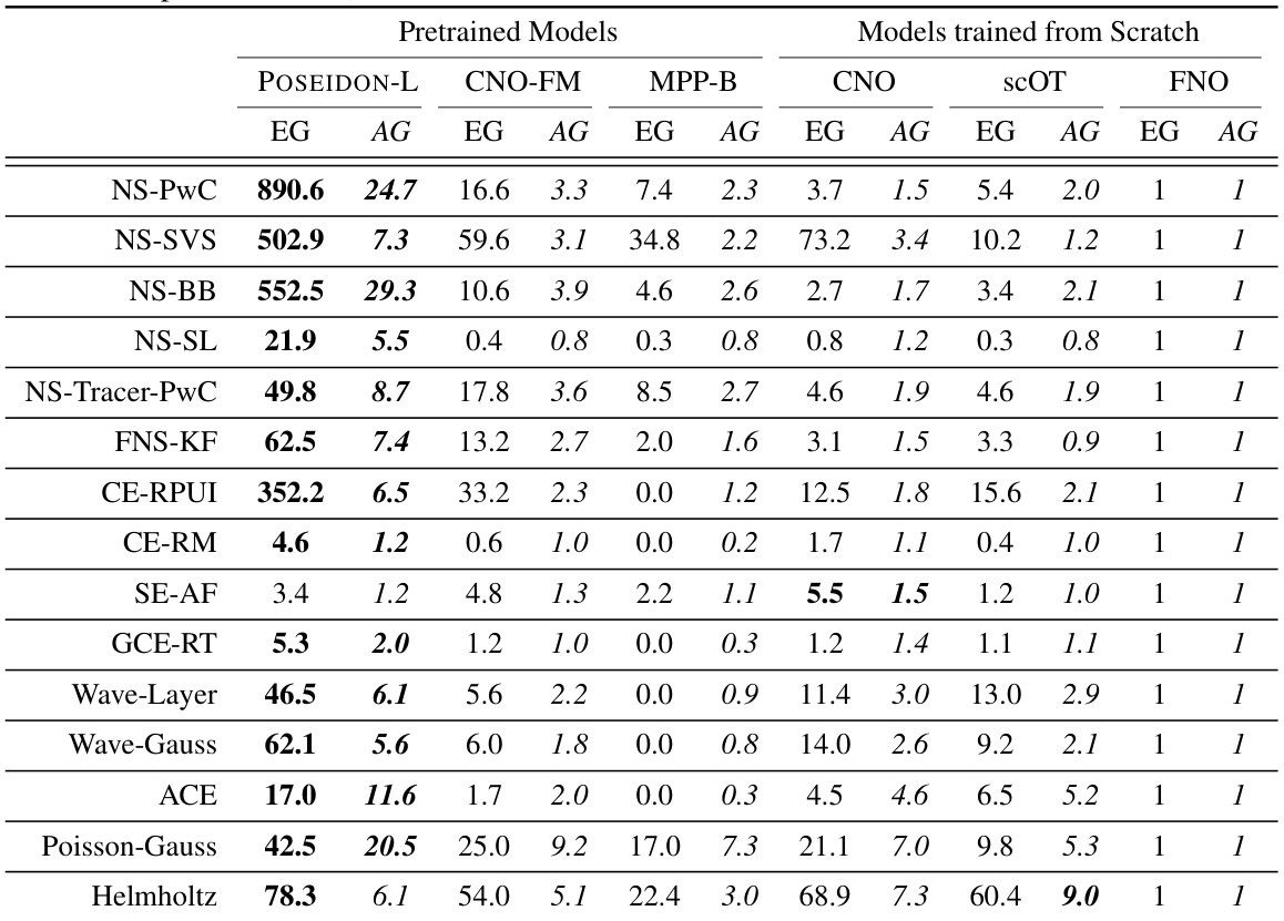
This table presents the efficiency and accuracy gains of different models (POSEIDON-L, CNO-FM, MPP-B, CNO, scOT, and FNO) on 15 downstream tasks. Efficiency gain (EG) measures how many fewer samples a model needs compared to FNO to achieve the same error level. Accuracy gain (AG) measures how much more accurate a model is than FNO for a given number of samples. The results highlight the superior performance of the POSEIDON models, especially in terms of sample efficiency.
In-depth insights#
PDE Foundation Models#
The concept of “PDE Foundation Models” represents a significant advancement in the field of scientific machine learning. It leverages the power of large language models to tackle the complexities of solving partial differential equations (PDEs). By pretraining a model on a diverse range of PDEs, a foundation model can learn robust and generalizable representations, overcoming the limitations of task-specific neural operators which require extensive training data. This approach results in improved sample efficiency, and better generalization to unseen PDEs, even those involving significantly different physical phenomena. Open sourcing the models and datasets is a crucial aspect of this work, fostering collaboration and further advancements in the field. However, challenges remain, including generalizing to more complex geometries and PDE types, and ensuring robustness to various data distributions and noise levels. Future research will need to focus on addressing these issues and on the exploration of potential societal impact of such powerful models.
Multiscale Operator#
A multiscale operator, in the context of a PDE (Partial Differential Equation) solver, is a powerful approach to handle problems exhibiting a wide range of spatial scales. It leverages multiple resolutions or levels of detail to efficiently capture both fine-grained and coarse-grained features of the solution. This is crucial because many real-world phenomena modeled by PDEs are inherently multiscale, with small-scale details impacting large-scale behavior. The core idea is to use a simplified representation at coarser scales, reducing computational complexity. At finer scales, more detail is provided to accurately represent the solution’s intricate features. This approach is particularly beneficial for solving computationally expensive PDEs, as it can substantially reduce the runtime without sacrificing the accuracy in the solution.
All2all Training#
The all2all training strategy, a core innovation in the POSEIDON model, significantly enhances sample efficiency by leveraging the semi-group property inherent in time-dependent PDEs. Instead of training on individual time steps, it utilizes all possible pairs of snapshots within a trajectory. This approach dramatically increases the effective training data size, particularly crucial for foundation models aiming for generalization across diverse PDEs. The computational cost scales quadratically with the number of snapshots, but strategies like subsampling can mitigate this. The effectiveness of all2all training hinges on the semi-group property, and its benefits are most pronounced in scenarios where data is scarce. While computationally more expensive than conventional methods, the significant gains in sample efficiency and accuracy strongly suggest that all2all training is a worthwhile approach for training effective and general-purpose PDE foundation models.
Unseen Physics#
The concept of “Unseen Physics” in the context of this research paper centers on the model’s capacity to generalize to physical phenomena not encountered during its pretraining phase. The model demonstrates a surprising ability to effectively handle PDEs and their underlying physical processes that significantly differ from the limited set of equations used for initial training. This generalization capability is highlighted by the model’s successful application to downstream tasks involving various PDE types, including those with unseen physical dynamics. The model’s capacity to extrapolate to unseen physics showcases the power of the underlying model architecture and training methodology. The results suggest the model has learned underlying principles applicable across a wide range of physical systems, rather than simply memorizing specific equation solutions. This capacity to transfer knowledge hints at the creation of a more general-purpose and efficient foundation model capable of addressing a broader range of physical problems. However, further research is needed to fully understand the mechanisms behind this impressive generalization capability. Future investigations could explore potential limitations of this generalization and provide deeper insights into the model’s learned representations.
Scalability and Limits#
A crucial aspect of any machine learning model is its scalability. The paper investigates the scalability of the POSEIDON model in terms of both its model size and the size of the training dataset. Larger models consistently outperform smaller ones, demonstrating improved accuracy and sample efficiency. Similarly, increasing the training dataset size leads to improved performance on downstream tasks, although this effect diminishes with larger datasets, implying potential diminishing returns in data size. The study also acknowledges inherent limits, such as the high computational cost associated with larger models and datasets. Further limitations include the challenge of generalizing to unseen physics and the restricted scope of PDEs considered during pretraining. Ultimately, the investigation highlights the trade-off between achieving better performance and managing the associated computational demands, indicating a need for further research to optimize training efficiency and explore more diverse datasets.
More visual insights#
More on figures
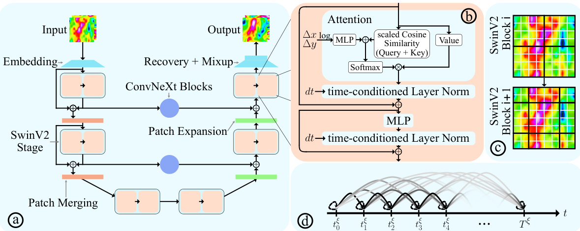
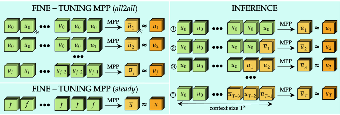
This figure details the architecture of the scOT model, a key component of POSEIDON. Panel (a) shows the overall hierarchical multiscale structure, combining SwinV2 Transformer blocks, ConvNeXt blocks, patch merging and expansion operations. Panel (b) zooms in on a single SwinV2 Transformer block, illustrating the multi-head self-attention mechanism with time-conditioned Layer Normalization. Panel (c) visualizes the sliding window approach used in the SwinV2 blocks, ensuring comprehensive attention across the spatial domain. Finally, panel (d) illustrates the novel ‘all2all’ training strategy employed for time-dependent PDEs, leveraging the semi-group property for enhanced data efficiency.
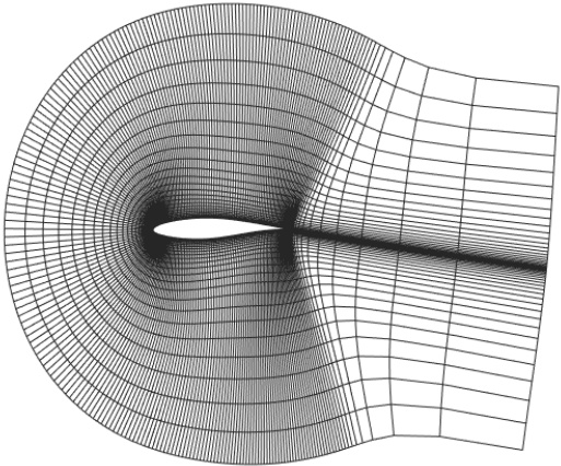
This figure shows the elliptic mesh used for the airfoil problem in the SE-AF downstream task. The mesh is a high-resolution grid that is designed to accurately resolve the flow around the airfoil. The mesh is particularly refined near the airfoil surface, where the flow is most complex. This is important for accurate simulation of the flow around the airfoil, particularly in the region near the trailing edge, where the flow is highly sensitive to small changes in the geometry. The mesh is generated using a standard elliptic grid generator. The SE-AF task involves solving the compressible Euler equations for flow around the RAE2822 airfoil shape. The solution operator maps the shape function to the density of the flow at steady-state. The figure visually depicts the mesh around the airfoil, highlighting the refinement in the area close to the body.

This figure illustrates the architecture of the Convolutional Neural Operator (CNO) model. It shows how the CNO is structured as a modified U-Net, utilizing a series of layers that map between bandlimited function spaces. The figure highlights the key components of the CNO architecture, including the lifting layer (P), downsampling and upsampling operations (D and U blocks), residual blocks (R blocks), invariant blocks (I blocks), convolutional and activation operators (K and Σ), and the projection layer (Q). The illustration helps to visualize the multi-scale and hierarchical nature of the CNO’s processing of functions.

This figure illustrates the finetuning procedure for the CNO-FM model. It shows two scenarios: in-context finetuning and out-of-context finetuning. In-context finetuning involves using the same input and output variables as in pretraining, while out-of-context finetuning uses different variables. Both scenarios involve adding a linear layer before the lifting layer and modifying the projection layer during finetuning. The diagram highlights the different components of the CNO model (lifting, base, projection) and how they are modified during the two finetuning scenarios.
The figure illustrates the sample efficiency of the POSEIDON model in comparison to PDE-specific operator learning methods. POSEIDON, a pretrained model, achieves comparable accuracy with significantly fewer training samples. It also demonstrates the model’s ability to generalize to previously unseen physical phenomena during fine-tuning.
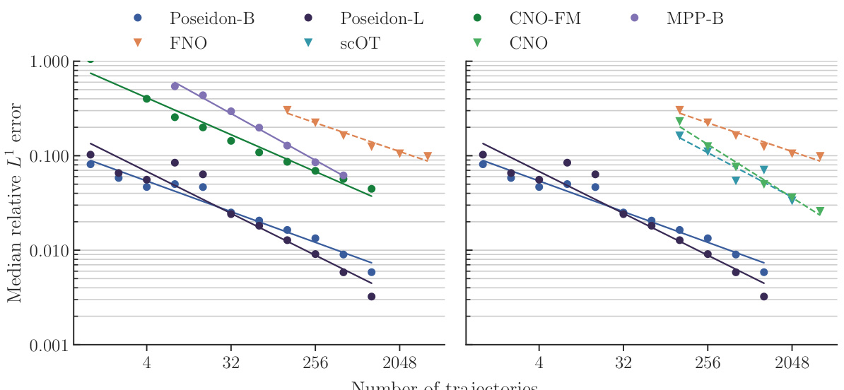
This figure displays the median relative L¹ error on the test set for the NS-PwC task, plotted against the number of trajectories used for training. Multiple models are compared: Poseidon-B, Poseidon-L, FNO, scOT, CNO-FM, CNO, and MPP-B. The graph shows how the error decreases as the number of training trajectories increases, illustrating the models’ performance and sample efficiency. The left panel emphasizes comparison between pretrained models. The right panel emphasizes comparison between models trained from scratch.
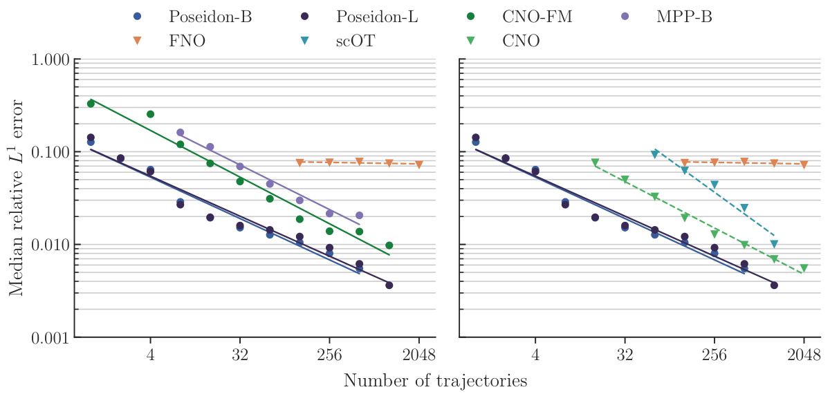
This figure displays the median relative L¹ error on the test set for the NS-PwC task, plotted against the number of trajectories used for training. It compares the performance of several models, including POSEIDON-B, POSEIDON-L, FNO, scOT, CNO, CNO-FM, and MPP-B. Each model’s performance is represented by a distinct line and color. The x-axis shows the number of trajectories, while the y-axis shows the error. The graph illustrates the sample efficiency and accuracy of different models in solving the NS-PwC problem. The purpose of the figure is to demonstrate the superior performance of the POSEIDON models compared to other methods.
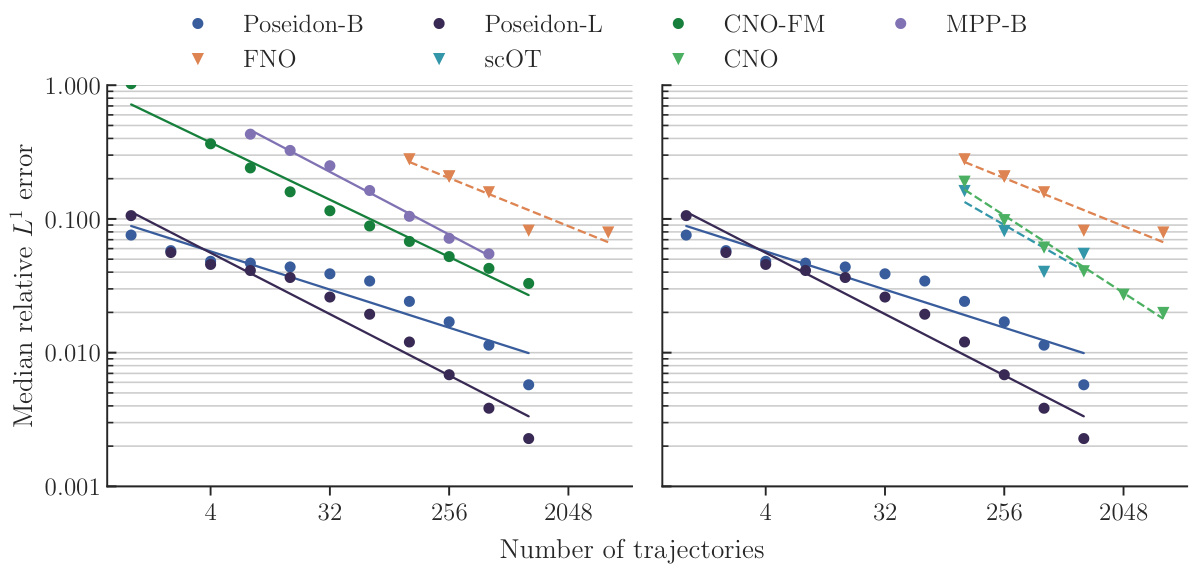
This figure presents the results of an experiment evaluating the performance of various models on the NS-PwC task. The x-axis shows the number of trajectories used for training, and the y-axis shows the median relative L¹ error on a test set. Multiple models are compared, including different sizes of the POSEIDON model, FNO, CNO, SCOT and MPP. The plot helps illustrate the sample efficiency and accuracy of the different models on this specific task. POSEIDON models, especially the larger ones, show better performance (lower error) with fewer training trajectories compared to the baselines.
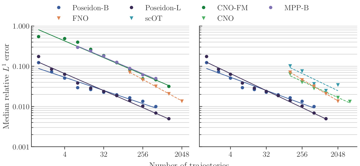
This figure displays the results of an experiment comparing the performance of various models on the NS-PwC task. The x-axis represents the number of trajectories used to train the models, and the y-axis represents the median relative L¹ error on a test set. The plot allows for a comparison of the sample efficiency and accuracy of different models, including the POSEIDON models (POSEIDON-B and POSEIDON-L), FNO, CNO, CNO-FM, and MPP-B. The lines represent the median error and the points show individual runs. This gives a clear picture of how the performance of each model scales with the amount of training data.
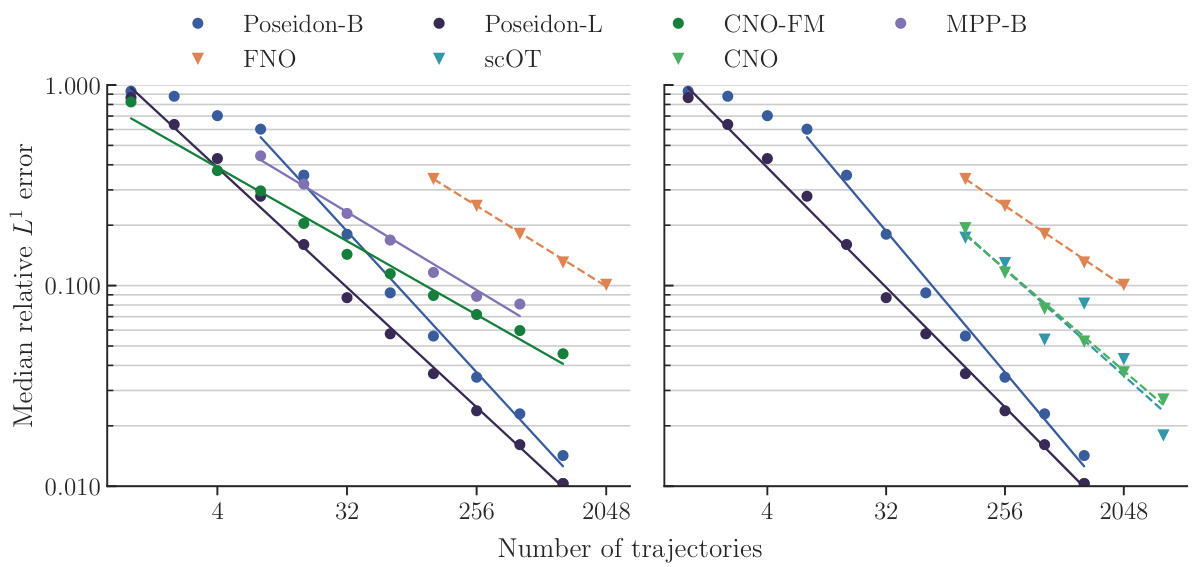
This figure displays the performance of different PDE solving models on the NS-PwC test dataset. The x-axis represents the number of trajectories used, and the y-axis shows the median relative L¹ error. The plot shows scaling curves for several models: Poseidon-B, Poseidon-L, FNO, SCOT, CNO-FM, and MPP-B. It demonstrates how the accuracy of these models improves as more trajectories are used for training. The figure illustrates the sample efficiency and accuracy of the models relative to one another.
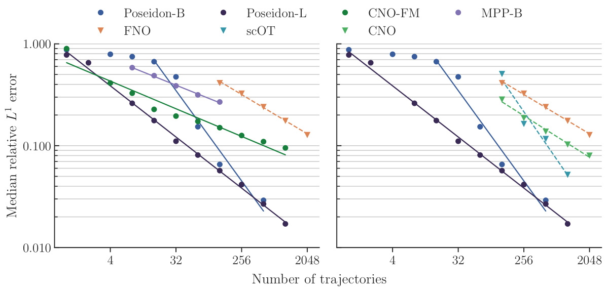
This figure displays the performance of various models on the NS-PwC (Navier-Stokes with Piecewise Constant Vorticity) task. The x-axis represents the number of trajectories used for training, and the y-axis shows the median relative L¹ error on the test set. Multiple models are compared: Poseidon-B, Poseidon-L, FNO, scOT, CNO-FM, and MPP-B. The plot shows how the error decreases as the number of training trajectories increases for each model, allowing for a comparison of their sample efficiency and accuracy.
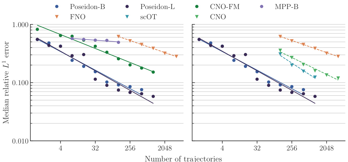
This figure displays the median relative L¹ error on the test set for the NS-PwC task (Navier-Stokes with Piecewise Constant Vorticity) as a function of the number of trajectories used for training. It compares the performance of several models: Poseidon-B, Poseidon-L, CNO-FM, MPP-B, FNO, scOT, and CNO. The graph shows how the error decreases as the number of training trajectories increases, demonstrating the impact of training data size on model accuracy. The different lines represent the performance of each model, highlighting the relative performance of each model in terms of sample efficiency and accuracy. The left and right subfigures present slightly different subsets of the models for improved visual clarity.

This figure presents the results of the NS-PwC experiment. It shows how the median relative L¹ error on the test set changes with respect to the number of trajectories used for training. The results for different models are plotted separately in this figure: POSEIDON-B, POSEIDON-L, CNO-FM, MPP-B, FNO, and CNO. The figure clearly shows how the error decreases as more trajectories are used for training and also shows that POSEIDON models outperforms other models, significantly.

This figure presents the results of the NS-PwC experiment, showing the relationship between the number of trajectories used for training and the median relative L¹ error on the test set for various models, including POSEIDON-B, POSEIDON-L, FNO, SCOT, CNO-FM, and MPP-B. The plot displays the scaling curves of the different models, revealing POSEIDON’s sample efficiency and accuracy gains compared to the baselines.

This figure displays the results of an experiment evaluating the performance of various models on the NS-PwC task. The x-axis shows the number of trajectories used to train each model, while the y-axis represents the median relative L¹ error on the test set. The models being compared include Poseidon-B, Poseidon-L, FNO, scOT, CNO-FM, CNO, and MPP-B. The plot illustrates how the error decreases as the number of training trajectories increases, showcasing the models’ sample efficiency and learning ability. The performance of POSEIDON models is notably better, showing significantly lower errors compared to other baselines at the same number of training trajectories. This highlights the superiority of the POSEIDON architecture and the effectiveness of its pretraining strategy.
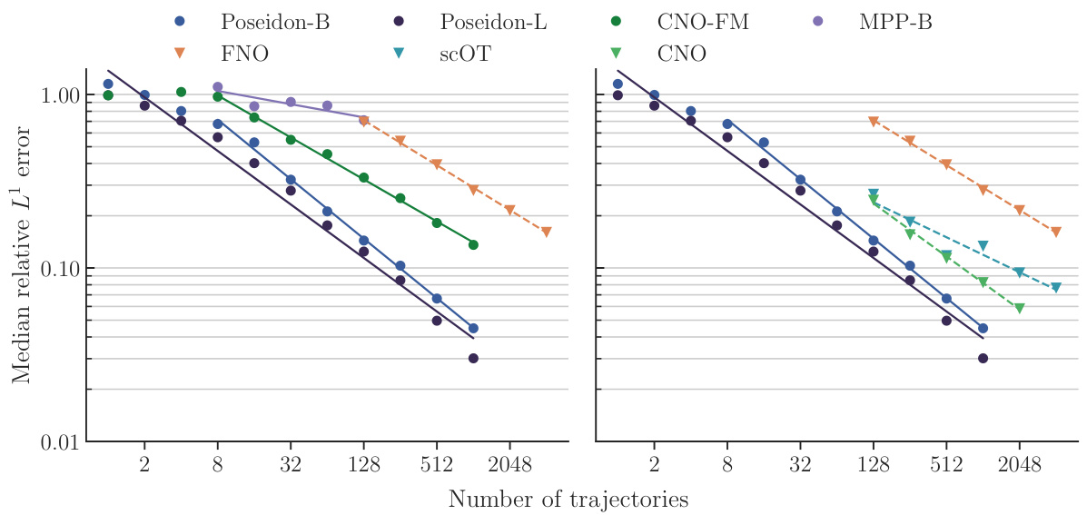
This figure presents the results of an experiment evaluating the performance of various models on the NS-PwC (Navier-Stokes with Piecewise Constant Vorticity) task. The x-axis represents the number of trajectories used to train each model, while the y-axis shows the median relative L¹ error on the test set. The models compared include different sizes of the POSEIDON model (POSEIDON-B and POSEIDON-L), FNO (Fourier Neural Operator), CNO-FM (pretrained CNO), MPP-B (Multiple Physics Pretraining), and scOT (scalable Operator Transformer). The plot shows the scaling curves for each model, illustrating how the median error decreases as the number of training trajectories increases. This visualization allows for a comparison of the sample efficiency and accuracy of each model on this specific task.

This figure displays the performance of various models on the NS-PwC task. The x-axis represents the number of trajectories used for training, while the y-axis shows the median relative L¹ error on the test set. Multiple models are compared, including various sizes of the POSEIDON model, along with FNO, CNO, SCOT, and MPP. The plot visually demonstrates the sample efficiency and accuracy gains of the POSEIDON model over the other baselines.
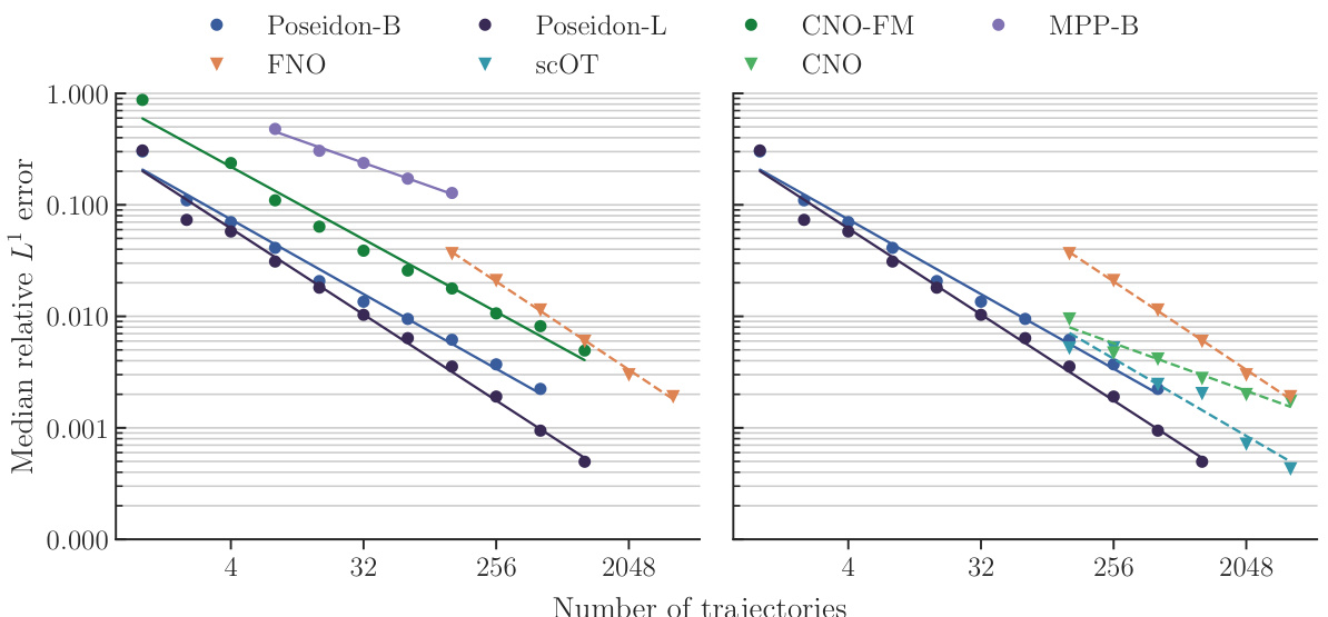
This figure displays the performance of different models on the NS-PwC downstream task by plotting the median relative L¹ error against the number of trajectories used for training. The models compared include POSEIDON-B, POSEIDON-L, FNO, scOT, CNO-FM, CNO, and MPP-B. The x-axis represents the number of training trajectories (log scale), and the y-axis represents the median relative L¹ error on the test set (log scale). The figure visually demonstrates the sample efficiency and accuracy gains of the POSEIDON models compared to the baselines. Specifically, it shows how many fewer trajectories POSEIDON requires to achieve a similar level of accuracy as the other models.
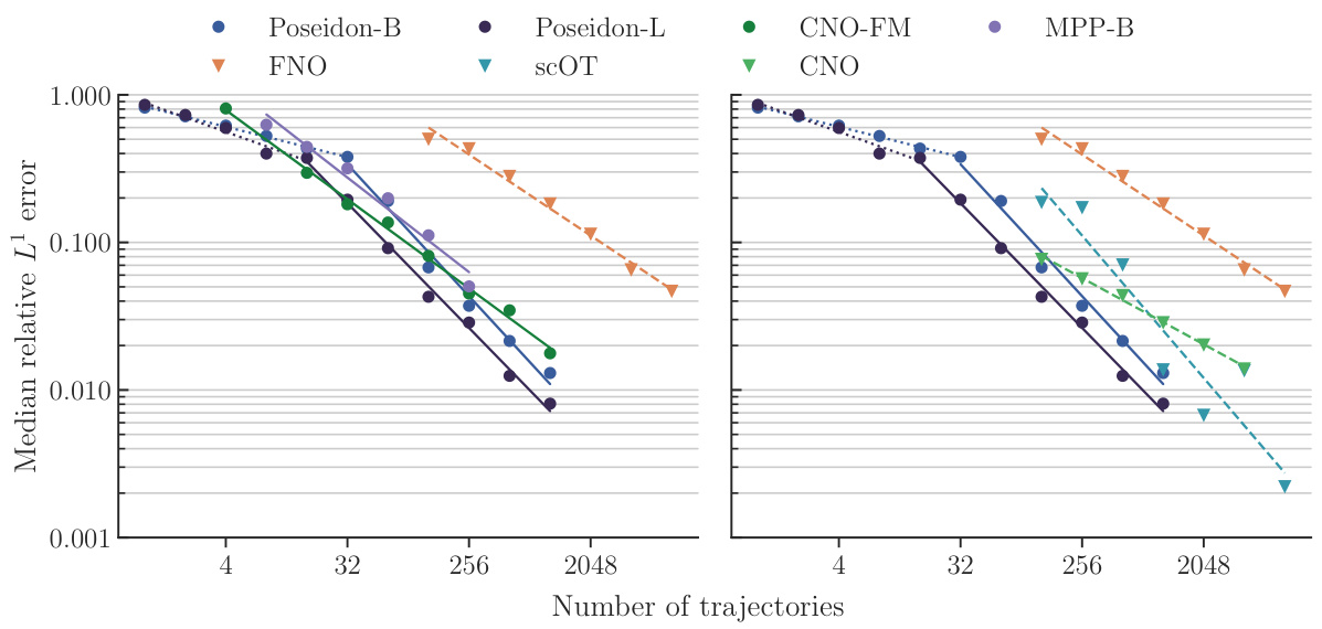
This figure displays the performance of various models on the NS-PwC task by plotting the median relative L¹ error against the number of trajectories used for training. The left panel shows the performance of the POSEIDON models (POSEIDON-B, POSEIDON-L) alongside CNO-FM and MPP-B, with FNO as a baseline. The right panel shows POSEIDON models and scOT, along with CNO and FNO. The x-axis represents the number of training trajectories while the y-axis represents the median relative L¹ error on the test set. This graph helps visualize sample efficiency and accuracy differences among different models.

This figure displays the performance of various models on the NS-PwC downstream task by plotting the median relative L¹ error against the number of trajectories used for training. It allows for a comparison of POSEIDON’s performance against several baseline models, including FNO, CNO, scOT, MPP-B, and a CNO foundation model. The figure shows the scaling curves, which illustrate how each model’s accuracy changes with increasing training data.
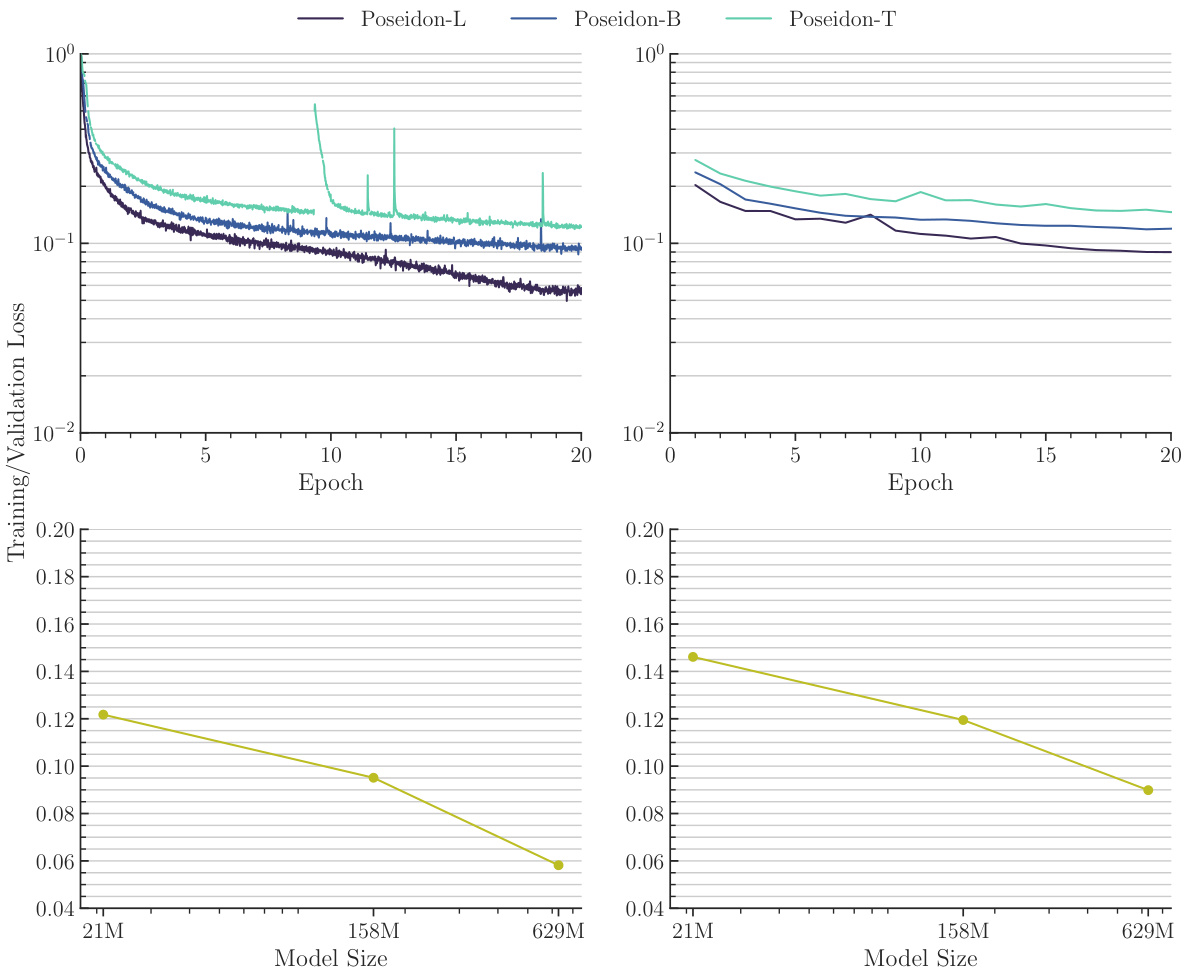
This figure shows the training and validation losses for different sizes of the Poseidon model during pretraining. The top row displays the loss curves over 20 epochs for three different model sizes: 21M, 158M, and 629M parameters. The bottom row presents the scaling of training and validation losses at epoch 20 as a function of model size. It visually demonstrates how the losses decrease with increasing model size.

This figure visualizes the impact of pretraining dataset size on model performance. The top section shows training and validation loss curves over 20 epochs for three dataset sizes: the full dataset, half the dataset, and one-eighth of the dataset. The bottom section displays the training and validation loss at epoch 20 for each dataset size. It demonstrates how increasing the dataset size leads to lower training and validation losses, indicating improved model performance.

This figure illustrates the architecture of the scOT model, which is the backbone of POSEIDON. It shows the SwinV2 Transformer block, the shifting window mechanism for multi-head self-attention, and the all2all training strategy for time-dependent PDEs. The scOT model is a hierarchical multiscale vision transformer with lead-time conditioning that processes lead time t and function space valued initial data input a to approximate the solution operator S(t, a) of the PDE (1).
This figure shows the training and validation loss curves for the POSEIDON-B model trained with different sizes of the pretraining dataset. The top row shows the training and validation loss curves for the model trained with the full, half and one-eighth sizes of the pretraining dataset. The bottom row shows the scaling of the training and validation losses at epoch 20 as a function of the number of trajectories used in pretraining.

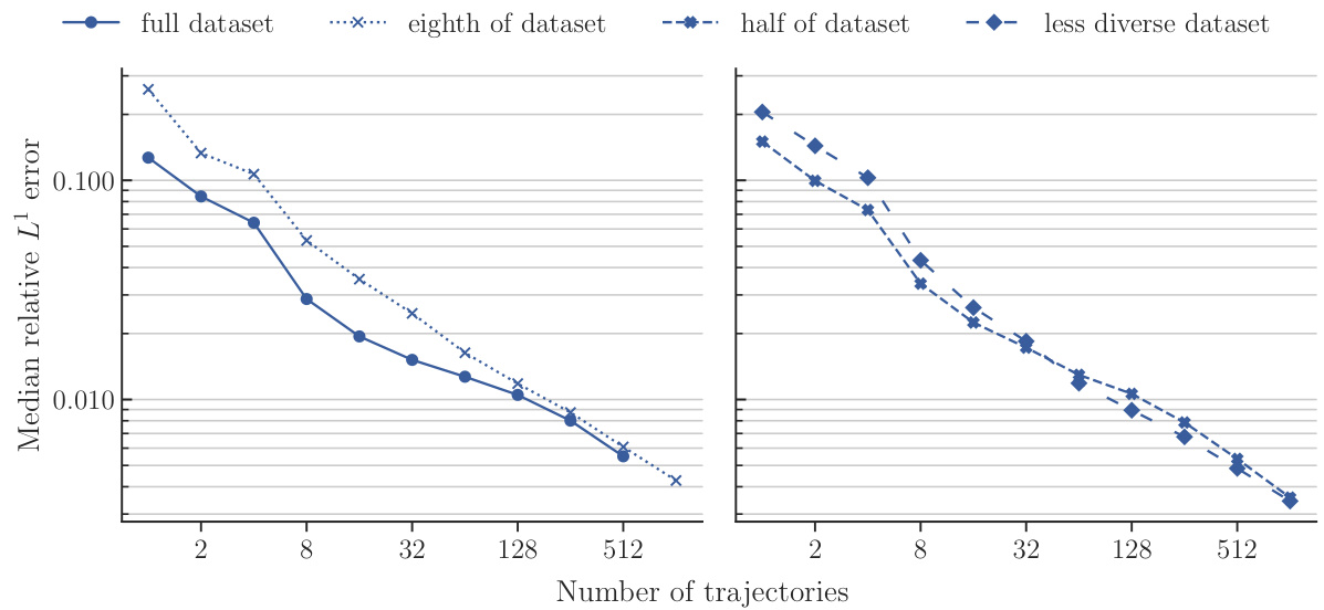
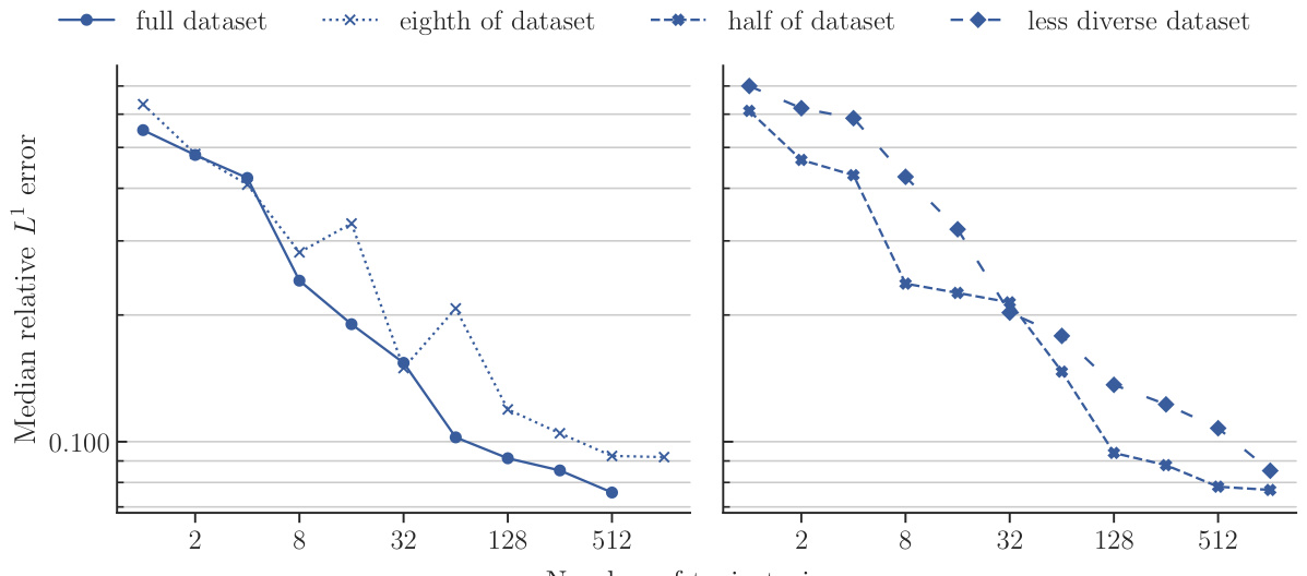
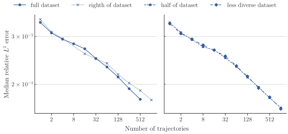
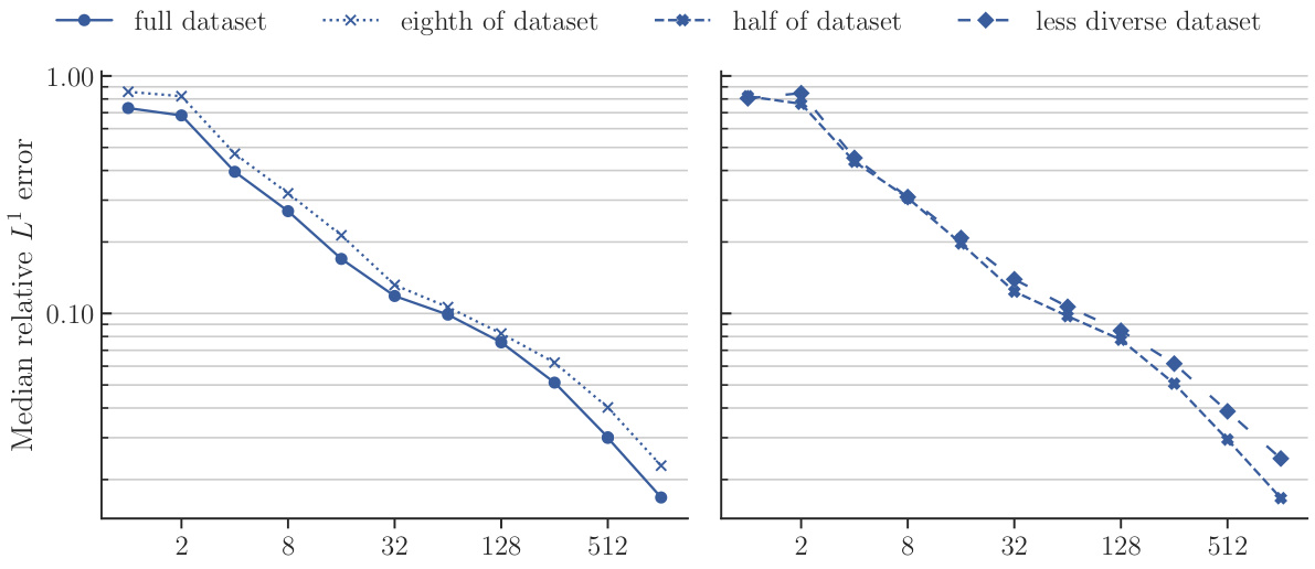
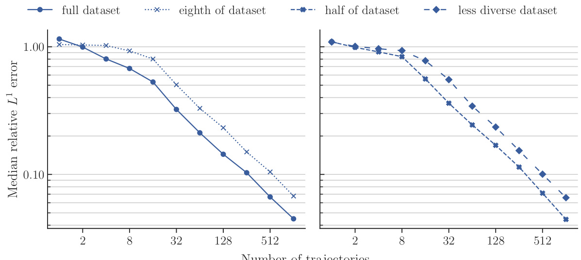
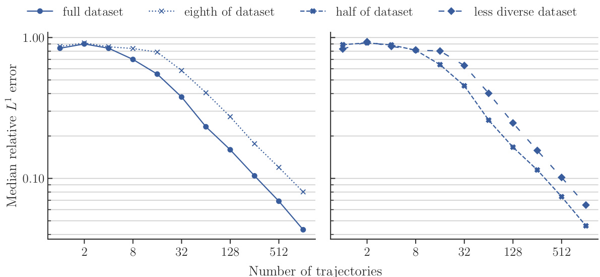
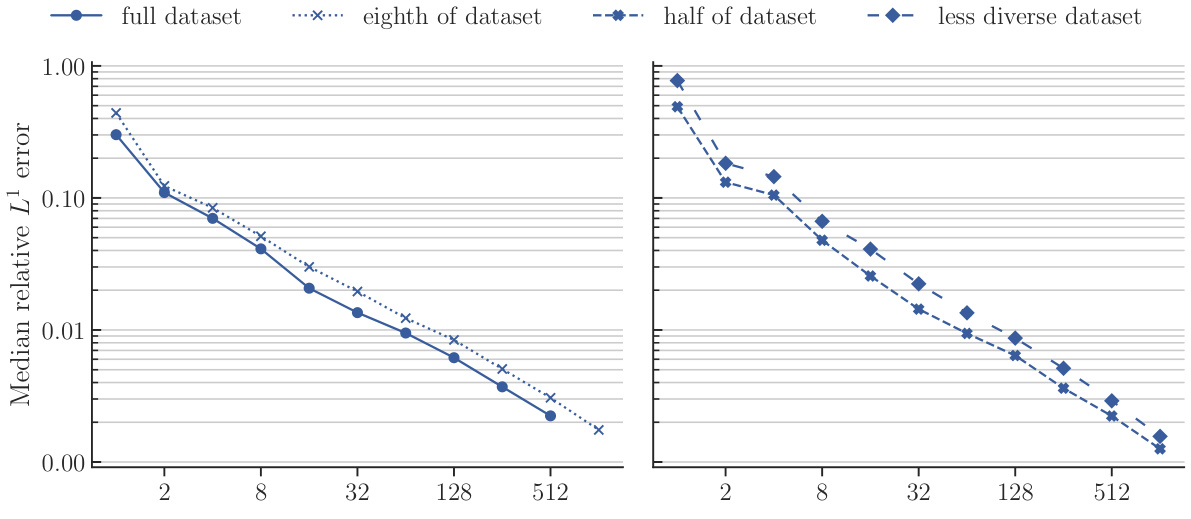
This figure compares the performance of POSEIDON-B trained with different sizes of the pretraining dataset on the NS-PwC downstream task. The left panel shows the performance of the model pretrained on the full dataset, one-eighth of the dataset, and half of the dataset. The right panel shows the performance of the model pretrained on half of the dataset and a less diverse dataset (where trajectories of 3 out of 6 operators are randomly removed). The plots show that the model trained on the full dataset performs best, followed by the model trained on half of the dataset. The model trained on a less diverse dataset has significantly worse performance. This demonstrates the importance of both quantity and diversity of the pretraining dataset for achieving high performance on unseen PDEs.

This figure shows how the training and validation losses during pretraining change with dataset size for the POSEIDON-B model. The top row displays the training and validation losses up to epoch 20 for different pretraining dataset sizes (one-eighth, one-half, and full size). The bottom row shows the scaling at epoch 20 for training loss (left) and validation loss (right).

This figure illustrates the architecture of the scOT model, a key component of POSEIDON. Panel (a) shows the overall hierarchical structure of scOT, which uses SwinV2 Transformer blocks and lead-time conditioning. Panel (b) details the structure of a SwinV2 Transformer block, highlighting the use of windowed multi-head self-attention. Panel (c) depicts the shifting window strategy used in the SwinV2 blocks. Finally, panel (d) visualizes the all2all training strategy used for time-dependent PDEs, which leverages the semi-group property of these PDEs to significantly increase the amount of training data.

This figure demonstrates the effect of pretraining dataset size on the performance of the POSEIDON-B model. The top section shows training and evaluation losses plotted against epochs for three different dataset sizes: the full dataset, half the dataset, and one-eighth of the dataset. The bottom section shows the scaling of training and evaluation losses at epoch 20, illustrating how these losses decrease with increasing dataset size.
This figure details the architecture of the scOT model, a hierarchical multiscale vision transformer used in POSEIDON. It shows the SwinV2 transformer block, the shifting window mechanism, and the all2all training strategy for time-dependent PDEs. The all2all strategy leverages the semi-group property of time-dependent PDEs for efficient training by using all possible data pairs within a trajectory. The SwinV2 block uses windowed multi-head self-attention, making it computationally efficient, and the windows are shifted across layers to ensure that all points in the domain are attended to.
This figure provides a detailed illustration of the scOT architecture, which is the foundation of the POSEIDON model. It’s broken down into four subfigures: (a) Shows the overall hierarchical multiscale architecture of scOT, highlighting the input embedding, SwinV2 transformer blocks, patch merging, patch expansion, and output reconstruction. (b) Zooms in on a single SwinV2 Transformer block, showcasing its components: the attention mechanism, MLP, and time-conditioned Layer Norm. (c) Illustrates the shifted-window attention mechanism used by SwinV2, where windows are shifted to allow all tokens to be considered. (d) Explains the all2all training strategy, where all possible pairs of snapshots from a trajectory are used to leverage the semi-group property of time-dependent PDEs to maximize training data and improve efficiency.

This figure shows the architecture of the scOT model, a key component of POSEIDON. Panel (a) presents the overall hierarchical multiscale structure of scOT, illustrating its encoder-decoder design with SwinV2 transformer blocks, patch merging, and patch expansion. Panel (b) zooms in on a single SwinV2 Transformer block, detailing its internal components: layer normalization, multi-head self-attention (MSA), and multi-layer perceptron (MLP). Panel (c) visualizes the shifting window mechanism used in the SwinV2 blocks, showing how windows are shifted across different layers to cover the entire input domain. Panel (d) illustrates the all2all training strategy, highlighting its effectiveness in leveraging trajectories of PDE solutions by using all possible data pairs (u(tk), u(t*)) with k ≤ k, in a single trajectory.
This figure illustrates the architecture of the scOT model, which is the backbone of POSEIDON. It shows the SwinV2 Transformer blocks, the shifting window mechanism, and the all2all training strategy used for time-dependent PDEs. Panel (a) provides a high-level overview of the scOT architecture. Panel (b) shows the details of the SwinV2 transformer block, which is a building block of the scOT. Panel (c) shows how the shifting windows are used to process the input tokens. Panel (d) illustrates the all2all training strategy, which is a novel strategy that allows for significant scaling-up of the training data.
This figure shows the training and validation losses for the POSEIDON-B model during pretraining with different dataset sizes (one-eighth, one-half, and full). The top row displays the training and validation loss curves up to epoch 20. The bottom row shows the training and validation losses specifically at epoch 20, illustrating the impact of dataset size on model performance during pretraining. The results demonstrate that the model’s performance improves as the training dataset size increases.
This figure shows how the training and validation losses of the POSEIDON-B model change with different sizes of the pretraining dataset. The top row presents the training and validation losses over 20 epochs for three different pretraining dataset sizes: one-eighth, one-half, and the full dataset. The bottom row displays the training and validation loss at epoch 20 for each dataset size, illustrating how the loss decreases with an increase in the size of the training data.
This figure shows the training and validation loss curves for the POSEIDON-B model trained with different sizes of the pretraining dataset. The top row displays the loss curves over time for the full, half, and one-eighth sizes of the pretraining dataset. The bottom row presents the training and validation loss at epoch 20 to illustrate the scaling behavior of the training with dataset size. It shows that smaller dataset sizes yield larger losses.
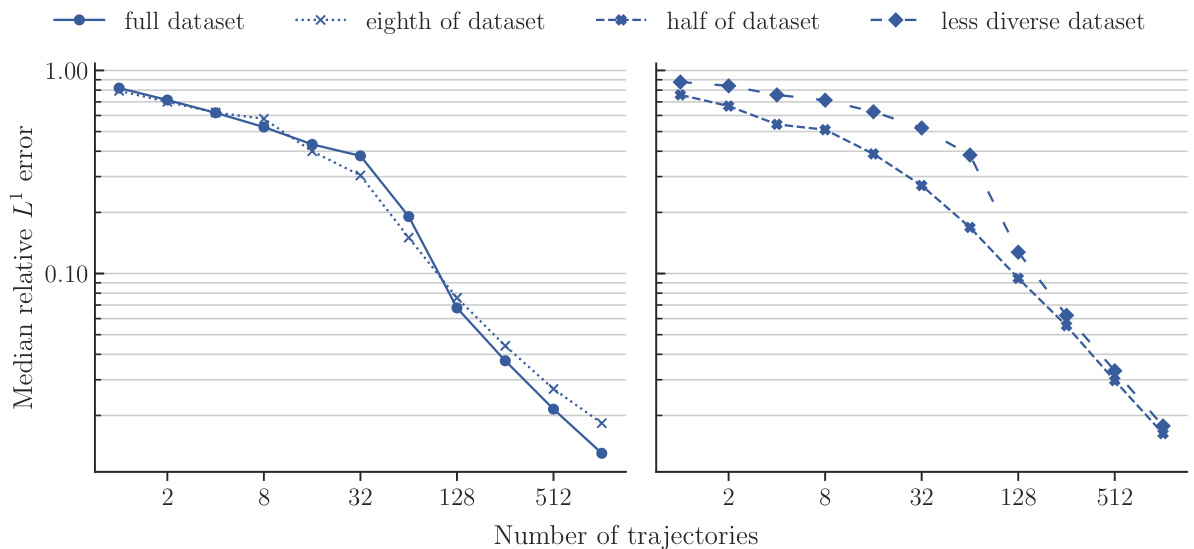
This figure displays the performance of four different models on the NS-PwC task in terms of median relative L¹ error against the number of trajectories used during training. The four training datasets compared are a ‘full dataset’, an ’eighth of dataset’, a ‘half of dataset’, and a ’less diverse dataset’. The graph shows how the accuracy of each model changes as more training data is provided, offering insights into sample efficiency and the impact of dataset size and diversity on model performance.
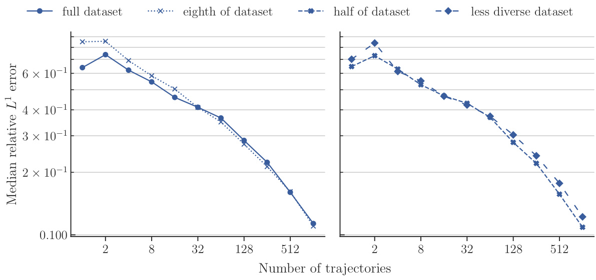
This figure displays the results of an experiment comparing the performance of POSEIDON-B trained on different sizes and diversities of the pretraining dataset on the NS-PwC downstream task. The x-axis represents the number of trajectories used for finetuning, and the y-axis shows the median relative L¹ error on the test set. Four lines are shown, corresponding to the full dataset, one-eighth of the dataset, half of the dataset, and a less diverse dataset (same size as half). The plot visually demonstrates how the model’s performance on the downstream task improves with the size and diversity of the pretraining dataset.

This figure visualizes how well POSEIDON-B generalizes to a unseen task with different numbers of task-specific training samples. The CE-RPUI task involves a complex solution with shocks and vortices. The figure shows that with only one task-specific sample, POSEIDON-B manages to capture some large-scale features of the solution, such as shock locations. With increasing number of samples (4, 32, and 128), the approximation gets better, and POSEIDON-B is able to capture even small-scale features. This illustrates how a foundation model for PDEs can leverage information learned from pre-training to quickly adapt to unseen physics with a few downstream samples.
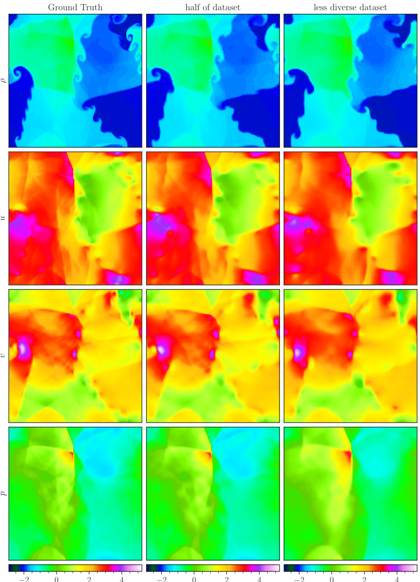
This figure shows a comparison of the CE-RPUI task’s approximation by the POSEIDON-B model when pretrained on different datasets. The leftmost column displays the ground truth of a random sample. The second and third columns illustrate the model’s performance when pretrained on half of the original training data and on a less diverse dataset, respectively. Visual comparisons of the density (ρ), horizontal velocity (u), vertical velocity (v), and pressure (p) across the three conditions reveal the impact of dataset size and diversity on the model’s ability to capture fine-grained details.

This figure shows how the POSEIDON-B model approximates a random sample from the CE-RPUI dataset when trained with different numbers of task-specific trajectories. The ground truth is shown in the first panel, followed by the model’s approximation with 1, 4, 32, and 128 trajectories, respectively. This demonstrates the model’s ability to improve its approximation accuracy with more training data. Each panel displays a color-coded representation of the solution, with the color intensity representing the magnitude of the solution. This figure provides a visual demonstration of the model’s sample efficiency in learning complex solution operators.

This figure visualizes how POSEIDON-B approximates a random sample from the CE-RPUI dataset when trained with varying numbers of task-specific trajectories. It showcases the model’s ability to improve its approximation as the number of training trajectories increases. The leftmost panel shows the ground truth. Subsequent panels display approximations with 1, 4, 32, and 128 trajectories. The visualization allows for a comparison of the model’s performance at different stages of finetuning, highlighting its improvement in accuracy as more task-specific data is provided.

The figure visualizes how POSEIDON-B’s approximation of a random sample from the Poisson-Gauss task improves with an increasing number of task-specific training samples. It showcases the model’s learning process, starting from a poor initial approximation (1 sample) to a much closer approximation that captures the main characteristics of the solution (512 samples). The color bar represents the values of the solution.

This figure displays a qualitative analysis of how well POSEIDON-B approximates a single random sample from the Poisson-Gauss test set with varying numbers of task-specific training samples. It demonstrates the model’s learning progression, starting with a poor approximation at 1 sample (mostly replicating the input), gradually improving towards a more accurate representation of the diffused and smoothed Gaussian features at 512 samples.
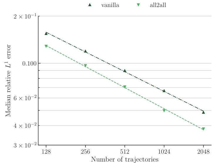
The figure compares the performance of the CNO model trained with the all2all training strategy against the vanilla training strategy for the NS-SL task. The all2all strategy leverages the semi-group property of time-dependent PDEs to significantly increase the amount of training data. The plot shows the median relative L¹ error on the test set versus the number of training trajectories. The results demonstrate that the all2all strategy leads to significantly better performance compared to the vanilla training strategy, indicating its effectiveness in improving sample efficiency and accuracy.

This figure demonstrates the impact of the all2all training strategy on the performance of CNO models for the NS-PwC task. The left panel shows the test errors when using different subsets of snapshots within a trajectory (T14, T7, T2), highlighting that denser sampling improves accuracy but with increasing computational costs. The right panel illustrates a saturation effect, showing that adding more samples beyond a certain point does not yield any significant accuracy improvements.

This figure compares the sample efficiency of POSEIDON with that of PDE-specific operator learning methods. It highlights that POSEIDON, a pretrained foundation model, requires significantly fewer samples to achieve comparable performance on downstream tasks (various PDEs). The figure visually emphasizes POSEIDON’s superior sample efficiency and its ability to generalize to unseen physics during finetuning.
This figure illustrates the architecture of the scOT model, the SwinV2 Transformer block, the shifting window mechanism, and the all2all training strategy for time-dependent PDEs. Panel (a) shows the overall hierarchical multiscale architecture of scOT, which is a U-Net style encoder-decoder using SwinV2 blocks. Panel (b) details the structure of a SwinV2 Transformer block, showing the windowed multi-head self-attention and MLP layers. Panel (c) visualizes how the shifting windows mechanism in the SwinV2 Transformer block works. Finally, Panel (d) depicts the all2all training strategy used to significantly increase the training data by leveraging the semi-group property of time-dependent PDEs.
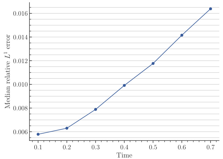
This figure displays the performance of various models on the NS-PwC task. It shows the median relative L¹ error on the test set plotted against the number of trajectories used for training. The models compared include Poseidon-B, Poseidon-L, FNO, scOT, CNO-FM, MPP-B, and CNO. The graph illustrates the sample efficiency of each model, showing how quickly their accuracy improves as more training data becomes available. This task assesses the models’ ability to solve Navier-Stokes equations with piecewise constant vorticity initial conditions. The trendlines help to visually determine the model’s rate of accuracy improvement with more training samples.

This figure compares the sample efficiency of POSEIDON, a pretrained foundation model, to PDE-specific operator learning methods. It shows that POSEIDON requires significantly fewer training samples to achieve similar accuracy compared to task-specific models. It also highlights the model’s ability to generalize to unseen physics, showcasing its effectiveness as a general purpose PDE solver.

This figure displays the training and validation losses for the POSEIDON models during the pretraining phase. The top part shows the training and validation losses up to epoch 20 for different model sizes (POSEIDON-T, POSEIDON-B, and POSEIDON-L). The bottom part demonstrates the scaling behavior of both training and validation losses at epoch 20 with respect to model size.

This figure shows the training and validation losses for different model sizes (POSEIDON-T, POSEIDON-B, POSEIDON-L) during the pretraining phase. The top row displays the training and validation loss curves over 20 epochs, demonstrating the decrease in both loss types as the model size increases. The bottom row presents a concise summary of the training and validation losses at epoch 20, emphasizing the performance improvement correlated with increased model size.
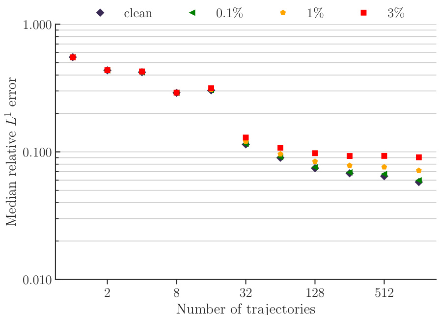
This figure displays the impact of adding Gaussian noise to the initial conditions of the CE-RPUI downstream task during the inference phase. Four different noise-to-signal ratios (NSRs) are tested: 0.1%, 1%, 3%, and a clean (no noise) condition. The median relative L1 error is plotted against the number of training trajectories used to finetune POSEIDON-L. The results showcase the model’s robustness to noise, even at a relatively high NSR of 3%, where the error remains reasonably low.
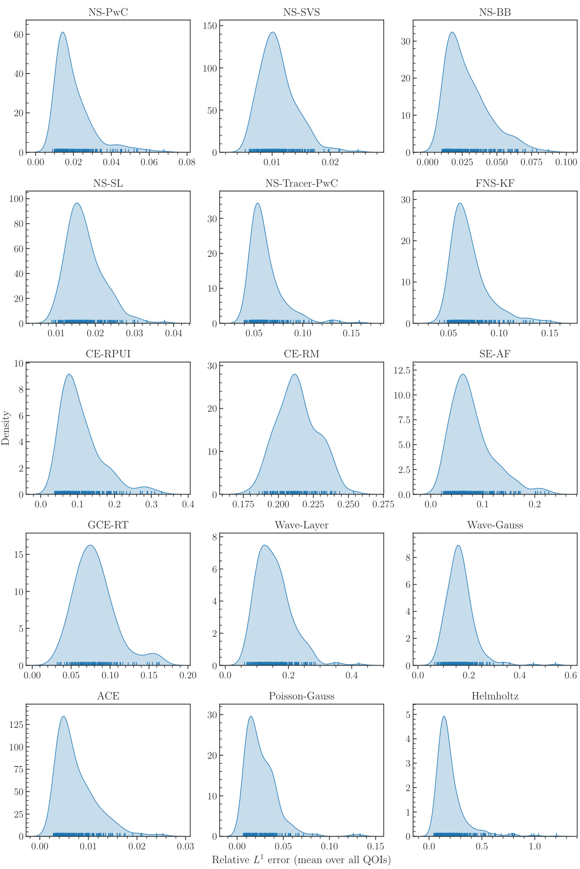
This figure presents kernel density estimations of the relative L1 error distributions for all 15 downstream tasks. Each plot corresponds to a specific task. The model POSEIDON-B is used with 128 and 512 trajectories for time-dependent and time-independent tasks, respectively. The x-axis represents the relative L1 error, and the y-axis displays the density. These plots help to visualize the performance variability across different downstream tasks and to understand the distribution of the errors.

The figure visualizes a random sample from the NS-Sines dataset. It shows a comparison between the ground truth (top) and samples predicted by POSEIDON-B at time T=1 (bottom). The left side shows the horizontal velocity (u), and the right shows the vertical velocity (v). The color scale represents the magnitude of the velocity.

This figure visualizes a random sample from the NS-Sines dataset. The top row shows the ground truth horizontal and vertical velocity fields, while the bottom row displays the corresponding predictions made by the POSEIDON-B model at time T=1. The color scheme represents the magnitude of the velocity fields, allowing for a visual comparison of the model’s performance in capturing the complex flow patterns.

This figure visualizes a random sample from the NS-Sines dataset. The top row displays the ground truth for the horizontal velocity (u) and vertical velocity (v). The bottom row shows the corresponding predictions generated by the POSEIDON-B model at the final time step (T=1). The color map represents the velocity magnitude, providing a visual comparison between the ground truth and model predictions. The figure demonstrates the model’s ability to accurately capture the complex features of the flow field, including the sine-wave-like structure of the initial condition.

The figure shows a comparison of the ground truth solution and POSEIDON-B’s approximation for a random sample of the CE-RPUI task using different numbers of task-specific trajectories. It showcases how the model’s accuracy improves with increasing finetuning data. The figure demonstrates POSEIDON-B’s ability to learn complex flow features (like shock waves and vortices) from only a few finetuning examples, highlighting the model’s sample efficiency.

This figure visualizes a random sample from the CE-RP (Compressible Euler - Riemann Problem) dataset used in the paper. The top row shows the ground truth values for density (ρ), horizontal velocity (u), vertical velocity (v), and pressure (p). Each variable is represented by a 2x2 grid of color-coded values. The bottom row displays the corresponding values predicted by the POSEIDON-B model after finetuning with 128 trajectories at time T=1. This demonstrates the model’s ability to approximate the complex dynamics represented in this particular Riemann problem, illustrating the model’s performance and the complexity of the data.
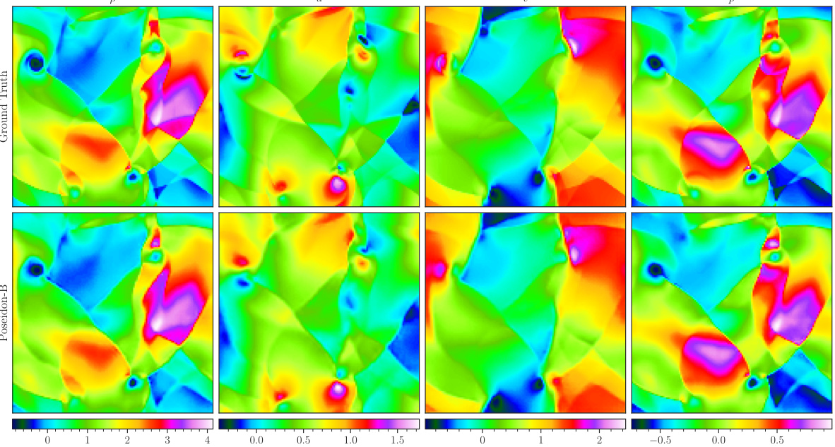
This figure visualizes how well POSEIDON-B approximates a single random sample from the CE-RPUI task when finetuned with different numbers of task-specific trajectories (1, 4, 32, 128). The top row shows the ground truth, while the subsequent rows display the model’s predictions with increasingly more trajectories. The results demonstrate the ability of POSEIDON-B to progressively refine its approximation with more data, capturing both large-scale features (like shock locations) and smaller-scale features (like vortex roll-ups) accurately.

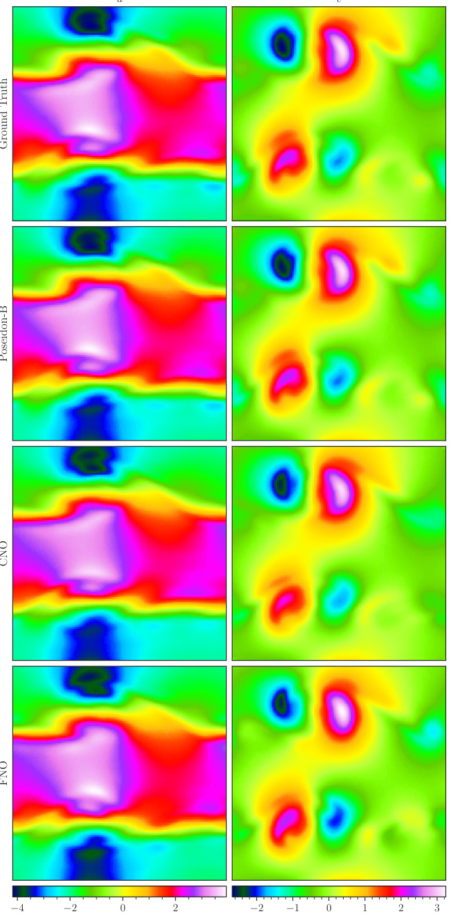
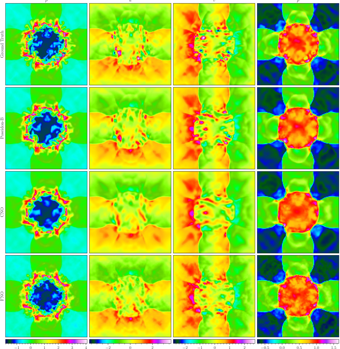
This figure visualizes a random sample from the CE-RP (Compressible Euler - Riemann Problem) dataset. The top row displays the ground truth data for density (ρ), horizontal velocity (u), vertical velocity (v), and pressure (p). The bottom four rows show how density, horizontal velocity, vertical velocity and pressure are predicted by the finetuned POSEIDON-B, CNO, and FNO models at time T=1. The image shows that POSEIDON-B exhibits a much better performance in capturing the shocks and vortices than CNO and FNO.

This figure displays a comparison of the CE-RPUI task’s results using two different POSEIDON-B models. The first model was pretrained using half of the original pretraining dataset, while the second was pretrained using a less diverse dataset. Each image shows the results for the ground truth data and the predictions made by each model for various samples. The figure demonstrates the impact of both dataset size and dataset diversity on the model’s performance.

This figure visualizes a random sample from the CE-RP (Compressible Euler Riemann Problem) dataset used in the paper. It shows the ground truth data and the predictions made by the POSEIDON-B model, CNO, and FNO models at a specific time (T=1). The input variables (density, horizontal velocity, vertical velocity, and pressure) are shown in the top row, with the ground truth and model predictions displayed in the bottom rows. The figure aims to demonstrate the accuracy of the POSEIDON model in capturing complex features such as shocks and vortices.
This figure visualizes a random sample from the NS-Sines dataset. The top row shows the ground truth data for the horizontal velocity (u) and vertical velocity (v). The bottom row presents the corresponding predictions generated by the POSEIDON-B model at time T=1. The color scheme represents the magnitude of the velocity components, allowing for a visual comparison between the ground truth and the model’s predictions. This dataset is characterized by sine initial conditions for the Navier-Stokes equations.

This figure visualizes a random sample from the NS-Sines dataset. The top row shows the ground truth data, with the horizontal and vertical velocity components displayed as input. The bottom row shows the samples predicted by the POSEIDON-B model at T=1.

This figure shows how well POSEIDON-B can approximate a random sample from the CE-RPUI task under different numbers of task-specific training trajectories. The top row displays the ground truth solution, while the subsequent rows show the model’s predictions when trained with 0, 1, 4, 32, and 128 task-specific trajectories, respectively. It demonstrates the model’s ability to progressively refine its approximation of the complex flow features (shocks and vortices) with increased training data.

This figure visualizes a random sample from the NS-Sines dataset. The top row shows the ground truth horizontal and vertical velocity fields (u and v, respectively). The bottom row presents the corresponding predictions made by the POSEIDON-B model at time T=1. The color bar indicates the range of values for the velocity fields.

This figure visualizes a random sample from the NS-Sines dataset. The top row shows the ground truth horizontal and vertical velocity fields. The bottom row displays the corresponding fields predicted by POSEIDON-B at time T=1. The color maps represent the magnitude of the velocities.
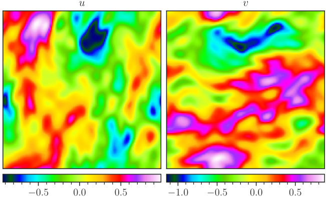
This figure visualizes a random sample from the NS-Sines dataset. The top row shows the ground truth horizontal velocity (u) and vertical velocity (v) fields. The bottom row displays the corresponding predictions made by the POSEIDON-B model after training on a single trajectory. The color maps represent the velocity magnitudes.

This figure visualizes a random sample from the NS-Sines dataset. It shows a comparison between the ground truth (top row) and the results predicted by the POSEIDON-B model at T=1 (bottom row). The left column displays the horizontal velocity (u), and the right column displays the vertical velocity (v). The color scale represents the magnitude of the velocity, highlighting differences in flow patterns between the ground truth and the model’s prediction.

The figure shows an elliptic mesh used for the airfoil problem in the SE-AF downstream task. The mesh is not uniform, with higher resolution near the airfoil surface to capture the fine details of the flow around the airfoil. The airfoil itself is defined using Hicks-Henne bump functions, allowing for variations in its shape. The mesh density is critical for accurately solving the steady-state compressible Euler equations in this computationally expensive task.
This figure shows the approximation of a random sample from the CE-RPUI dataset by the POSEIDON-B model. It demonstrates how the model’s approximation improves as more task-specific trajectories are used during training. The figure showcases the ground truth solution alongside approximations generated with 0, 1, 4, 32, and 128 task-specific trajectories. It highlights how a foundation model can learn effective representations from a limited set of training data. The visualization helps in understanding how the model learns from pretraining and then leverages this knowledge for improving accuracy during finetuning.

This figure visualizes a random sample from the NS-Sines dataset. It shows the ground truth and the samples predicted by POSEIDON-B at T=1 for the horizontal and vertical velocity components. The visualization helps illustrate the model’s ability to capture complex flow patterns and the overall accuracy of its predictions.

This figure visualizes how POSEIDON-B approximates a random sample from the CE-RPUI task when trained with different numbers of task-specific trajectories. It shows the ground truth solution alongside the approximations generated by POSEIDON-B trained with 0, 1, 4, 32, and 128 task-specific trajectories. The visualizations allow for a comparison of the model’s performance with varying amounts of finetuning data, illustrating its ability to learn and generalize from limited task-specific samples. It demonstrates the capabilities of the model in capturing intricate features and dynamics of the underlying PDE.

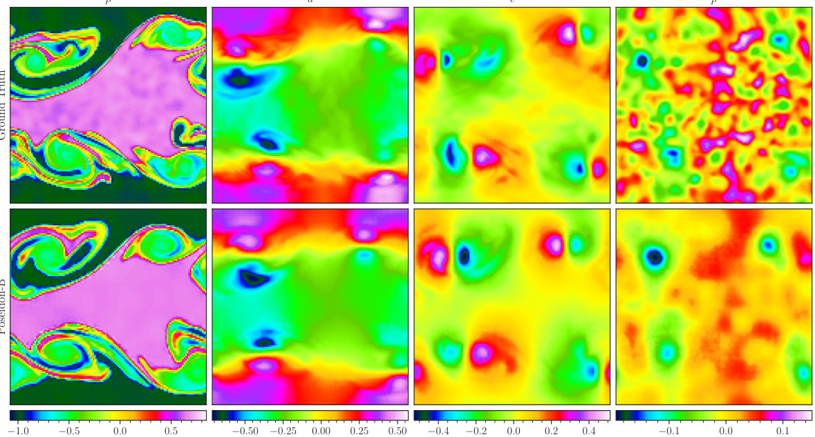
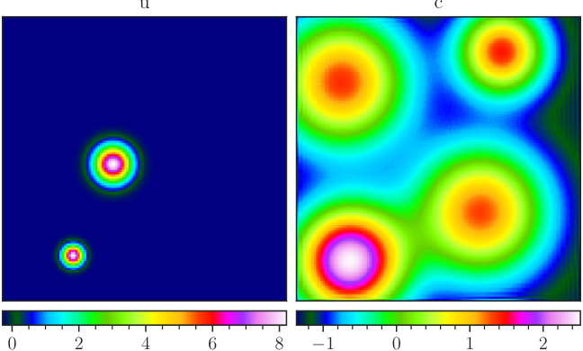
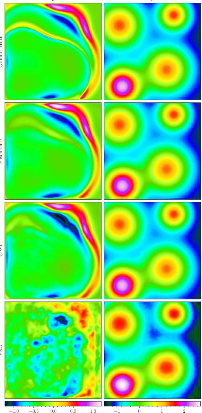
This figure visualizes a random sample from the NS-Tracer-PwC dataset. It shows the ground truth (top row) and predictions made by POSEIDON-B, CNO, and FNO (trained on 128 trajectories) at time T = 0.7. The inputs are the horizontal velocity (u), vertical velocity (v), and tracer concentration (c). The predictions of POSEIDON-B are much closer to the ground truth in comparison to CNO and FNO, demonstrating its effectiveness in capturing the complex flow and tracer dynamics.
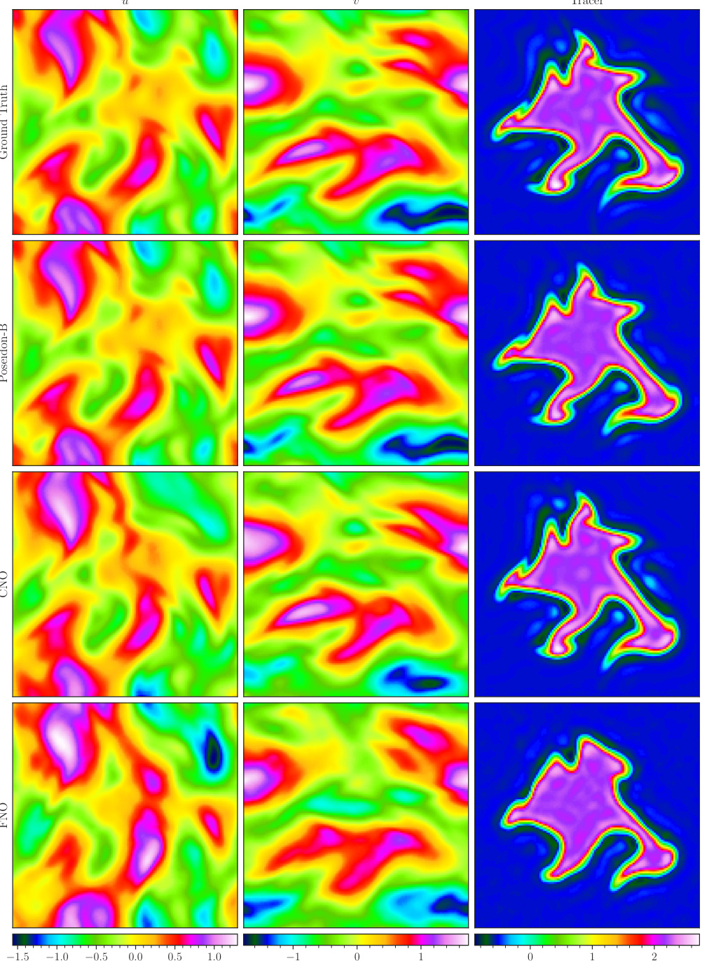
This figure visualizes a random sample from the NS-Tracer-PwC dataset at time T=0.7. It shows the ground truth (top row) and predictions made by POSEIDON-B, CNO, and FNO (trained on 128 trajectories) for the horizontal velocity u, vertical velocity v, and tracer concentration c. This task is out-of-distribution because it involves a passive tracer transport not explicitly present in the pretraining dataset. The figure demonstrates POSEIDON’s ability to generalize and provide accurate predictions even to unseen physics with limited training data. The comparison highlights the superior accuracy of POSEIDON-B.

This figure visualizes a random sample from the FNS-KF (Forced Navier-Stokes-Kolmogorov Flow) downstream task. It shows the ground truth and predictions made by three different models at T=0.7 (POSEIDON-B, CNO, and FNO). The inputs are horizontal velocity (u), vertical velocity (v), and forcing term (f). The figure illustrates the models’ ability to capture the complex flow features generated by the Kolmogorov flow forcing.
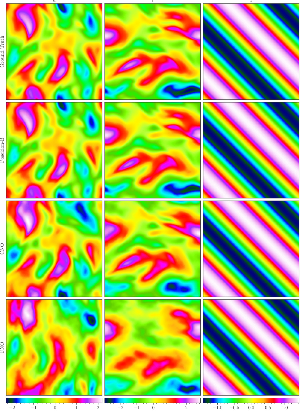
This figure visualizes a random sample from the Helmholtz downstream task. The top row shows the ground truth, while subsequent rows depict the samples predicted by the finetuned POSEIDON-B, CNO, and FNO models at the 14th time step. The inputs are the propagation speed (f), and the outputs are the solution (u). This demonstrates the models’ ability to approximate solutions to this task, highlighting the performance differences between the models.

This figure shows the elliptic mesh used for solving the flow around airfoil problem. The upper and lower surfaces of the airfoil are located at (x, yuf(x/c)) and (x, ylf(x/c)) respectively, where c is the chord length and yu and yl correspond to the well-known RAE2822 airfoil. The reference shape is then perturbed by Hicks-Henne Bump functions. The figure provides a visual representation of the computational mesh utilized to simulate the steady-state solution of the compressible Euler equations. The mesh density is higher around the airfoil to accurately capture flow details. The details of how the mesh is generated and the boundary conditions applied are discussed in the paper.
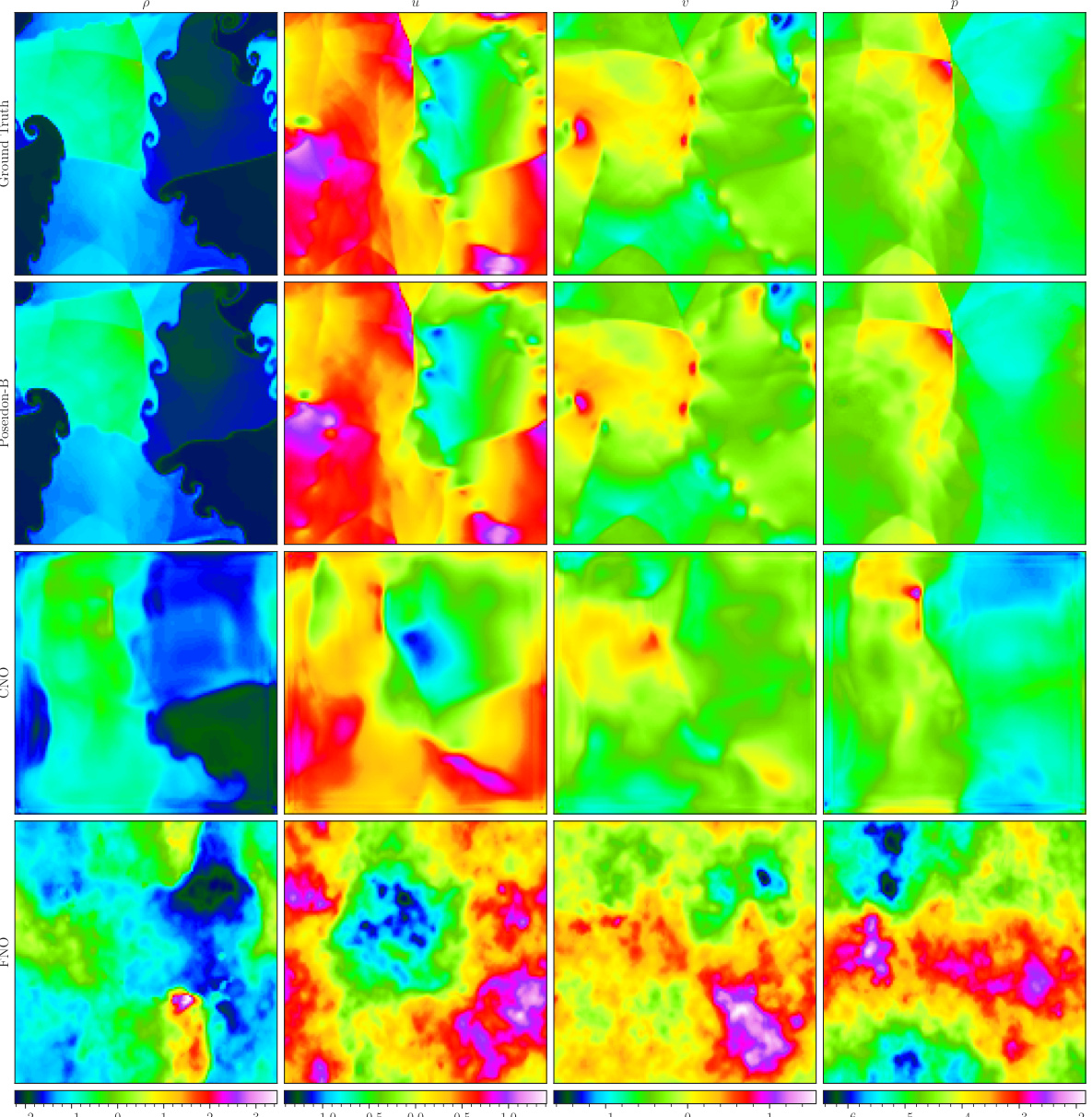
This figure visualizes a random sample from the CE-RPUI (Compressible Euler equations with uncertain interfaces) dataset. It shows the ground truth and the predictions made by POSEIDON-B, CNO, and FNO at time T=0.7. Each model’s prediction is displayed in a separate row, and the ground truth is shown in the top row. The figure shows the density, horizontal velocity, vertical velocity and pressure.

This figure visualizes a random sample from the CE-RM (Richtmeyer-Meshkov) dataset, showing the ground truth and predictions made by the three POSEIDON models (POSEIDON-L, POSEIDON-B, POSEIDON-T), the CNO, and the FNO at time T = 1.4. The inputs are density, horizontal velocity, vertical velocity, and pressure. The output is the density.
This figure displays kernel density estimations of the error distributions obtained by evaluating the POSEIDON-B model on all 15 downstream tasks with 128 (time-dependent) and 512 (time-independent) samples. Each plot represents the distribution of the mean relative L¹ error for different tasks, offering a visual assessment of the model’s performance consistency and variability across various PDE types and complexities.

This figure visualizes a random sample from the GCE-RT (Compressible Euler equations with gravitation, Rayleigh-Taylor) downstream task dataset. It shows the ground truth data and the predictions made by the finetuned POSEIDON-B, CNO, and FNO models at the seventh time step. The inputs are density, horizontal velocity, vertical velocity, pressure, and gravitational potential. The visualization highlights the model’s ability (or lack thereof) to capture complex features of the simulation, such as the mixing and instability of the fluids.

This figure displays kernel density estimates of the relative L1 error for all downstream tasks in the paper. The model used is POSEIDON-B, finetuned on 128 trajectories for the time-dependent and 512 for the time-independent tasks. The error is calculated using the mean over all the quantities of interest for each task.
This figure visualizes a random sample from the Helmholtz downstream task. The top row shows the ground truth for the inputs (propagation speed) and the predicted outputs (solution) by the finetuned POSEIDON-B, CNO, and FNO models at the 14th time step. The inputs represent a spatially varying propagation speed, and the output is the solution to the Helmholtz equation under Dirichlet boundary conditions. The figure demonstrates the models’ ability to learn the complex wave patterns associated with the Helmholtz equation, showcasing both their accuracy and their ability to generalize to unseen examples.
This figure displays kernel density estimates of the relative L¹ error for each downstream task when using the POSEIDON-B model. The model is fine-tuned with 128 trajectories for time-dependent tasks and 512 trajectories for time-independent tasks. Each plot shows the error distribution for a specific task, providing insights into the model’s performance variability across different problem instances. The error is calculated over the mean of all functions or quantities of interest for each task.

This figure visualizes a random sample from the NS-Sines dataset. The top row shows the ground truth horizontal and vertical velocity fields (u and v respectively) at a specific time step (T=1). The bottom row shows the corresponding fields predicted by the POSEIDON-B model, also at T=1. This illustrates the model’s ability to learn and reproduce complex flow patterns from the NS-Sines dataset. The color scale represents the magnitude of the velocity.

This figure visualizes how well POSEIDON-B approximates the CE-RPUI task when trained with different numbers of task-specific samples. The left column shows the ground truth. The following columns show the approximation made by the model when trained with 0, 1, 4, 32, and 128 task-specific samples, respectively. As can be seen, the approximation accuracy increases significantly with the number of task-specific training samples. This experiment shows how a foundation model for PDEs can learn effective representations from its pretraining phase.

The figure visualizes a random sample from the NS-Sines dataset. It shows the ground truth (top) and the predictions made by POSEIDON-B at time T=1 (bottom). The left-hand side displays the horizontal velocity component (u), and the right-hand side displays the vertical velocity component (v). The color bar indicates the range of values for these velocity components.

This figure visualizes a random sample from the Helmholtz dataset and compares the ground truth solution with the predictions made by the finetuned POSEIDON-B, CNO, and FNO at the 14th time step. The input to the models is the propagation speed, and the output is the solution to the Helmholtz equation. The figure shows that POSEIDON-B provides a much more accurate approximation of the solution compared to the other methods, especially at finer scales. This highlights POSEIDON’s ability to generalize to different types of PDEs and data distributions.
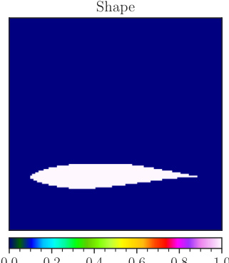
This figure displays the elliptic mesh used for the airfoil problem in the SE-AF downstream task. The mesh is a high-resolution grid used to numerically solve the compressible Euler equations around an airfoil. The airfoil shape is defined using Hicks-Henne bump functions. The image shows the grid resolution and its distribution around the airfoil, highlighting the refinement near the airfoil surface to accurately capture the flow features.

This figure visualizes a random sample from the Helmholtz dataset. It shows the ground truth solution and the predictions made by three models: POSEIDON-B, CNO, and FNO. Each model’s predictions are shown across multiple time steps. The figure showcases the ability of the models to approximate the solution of this complex partial differential equation.

This figure visualizes a random sample from the Poisson-Gauss dataset. The top panel shows the source term f, which is a superposition of Gaussians. The bottom panel shows the corresponding solution u predicted by POSEIDON-B, CNO, and FNO, each finetuned with 128 samples. The figure demonstrates the ability of the models to learn the solution operator which maps the source term f to the solution u, where the homogeneous Dirichlet boundary conditions are used. The model outputs are compared against the ground truth.

This figure visualizes a random sample from the Poisson-Gauss dataset, comparing the ground truth solution with the predictions made by POSEIDON-B, CNO, and FNO at the final time. The input is the source term which is a superposition of a random number of Gaussians. The solution is the output which is a diffused version of the source term, which respects Dirichlet boundary conditions.
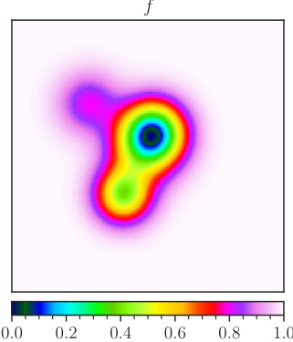
This figure visualizes a random sample from the Poisson-Gauss dataset. The top panel shows the source term (f), which is a superposition of Gaussians. The bottom panel presents the solution (u) obtained using different methods (POSEIDON-B, CNO, FNO) at various time steps. The figure illustrates the ability of the models to approximate the diffusion and smoothing properties of the Poisson equation, where the source term (f) is spread (diffused) and smoothed in the solution (u). The ground truth solution is shown at the top, alongside predictions made using the three different models.

This figure visualizes a random sample from the Poisson-Gauss dataset. It compares the ground truth solution to the solutions predicted by POSEIDON-B, CNO, and FNO, each trained on 128 trajectories. The ground truth displays a smooth diffusion of several Gaussians, while the predictions showcase varying degrees of accuracy in capturing this diffusion and smoothing effect.
More on tables
This table presents the scaling exponents obtained by fitting power laws to the scaling plots of different models on various downstream tasks. The power law equation used is of the form Emodel(M) ≈ CmodelM−amodel, where M represents the number of trajectories (or samples), Cmodel is the model-specific scaling factor, and amodel is the scaling exponent. The table shows that all models largely follow this scaling law, though with differing exponents for different tasks, indicating varying sample efficiency across different tasks and models.

This table summarizes the six datasets used for pretraining the POSEIDON model. It lists the abbreviation used in the paper for each dataset, the specific partial differential equation (PDE) that the dataset is based on (with equation number references from the paper), a key defining feature of each dataset (relating to the type of initial conditions used), and finally a figure reference to a visualization of the dataset in the supplementary materials.

This table summarizes the 15 downstream tasks used to evaluate the performance of POSEIDON and other models. Each task involves a different partial differential equation (PDE) and/or physical process. The table provides the abbreviation used for each task, the specific PDE involved, key defining features (e.g., initial conditions, forcing terms), and the figure number where a visualization of the task can be found. The (*) indicates that the solution for those tasks depends on the PDE parameters, sources or coefficients.

This table presents the efficiency and accuracy gains of various models (POSEIDON-L, CNO-FM, MPP-B, CNO, scOT, and FNO) across fifteen downstream tasks. The efficiency gain (EG) indicates how many fewer samples a model needs to reach the same error level as FNO, while the accuracy gain (AG) shows how much more accurate a model is than FNO for a given number of samples. Both EG and AG are calculated using the scaling curves generated in the paper. The values help to compare the sample efficiency and accuracy of different models on diverse PDE problems.
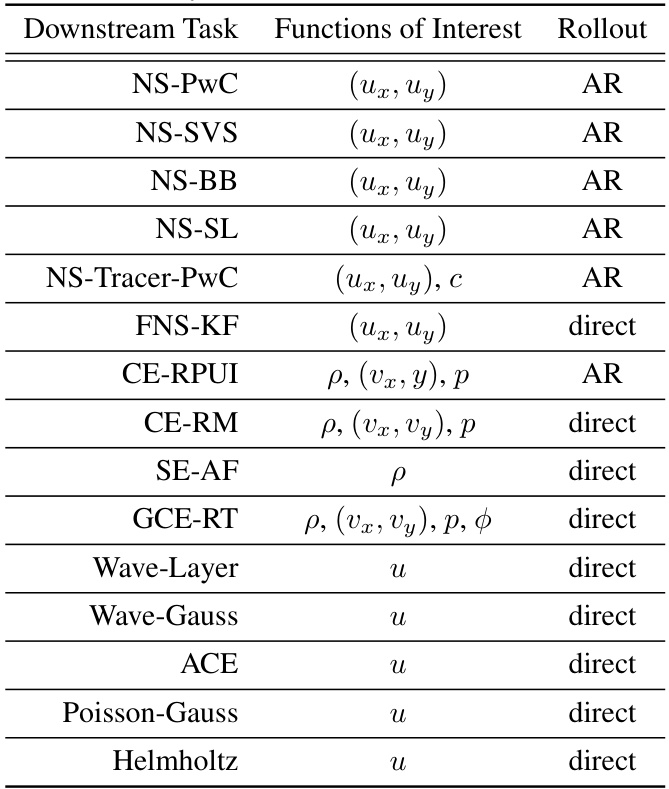
This table shows what quantities are used to calculate the relative L1 error for each downstream task. The ‘Functions of Interest’ column lists the specific variables (e.g., velocity components, density, pressure) used in the error calculation for each task. The ‘Rollout’ column indicates whether the solution is computed directly at the final time or using an autoregressive (AR) approach, which involves predicting the solution at successive time points.
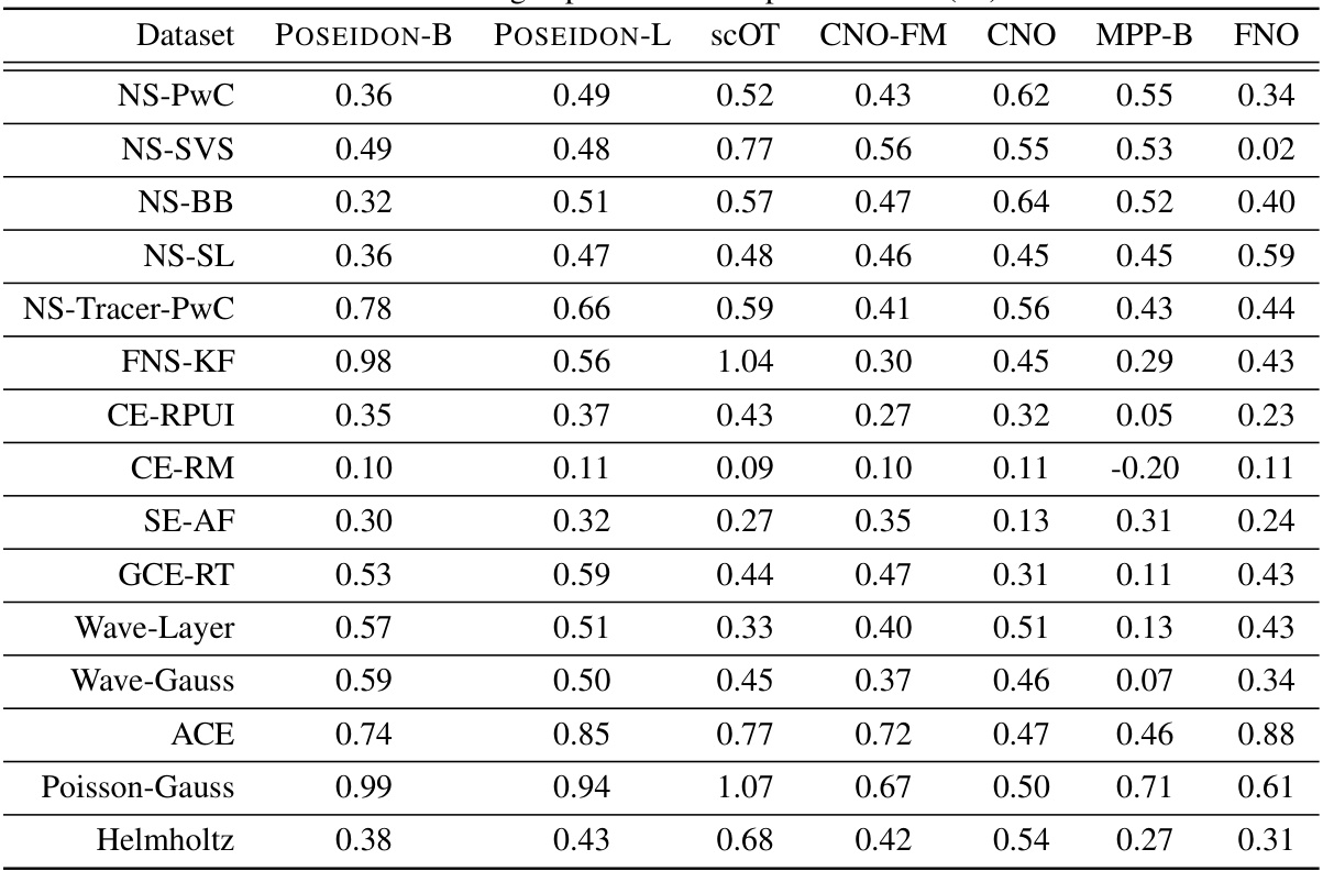
This table shows the scaling exponents obtained by fitting power laws to the scaling plots (Figures 7-21) in Section D.1 of the paper. The scaling exponents reflect how the median relative L¹ error changes with the number of trajectories (for time-dependent PDEs) or samples (for time-independent PDEs) for each of the models (POSEIDON-B, POSEIDON-L, scOT, CNO-FM, CNO, MPP-B, and FNO) across different downstream tasks. The table provides insights into the sample efficiency of each model. Note that the scaling exponent is just one part of the power law, the coefficient also plays a role in the actual error.
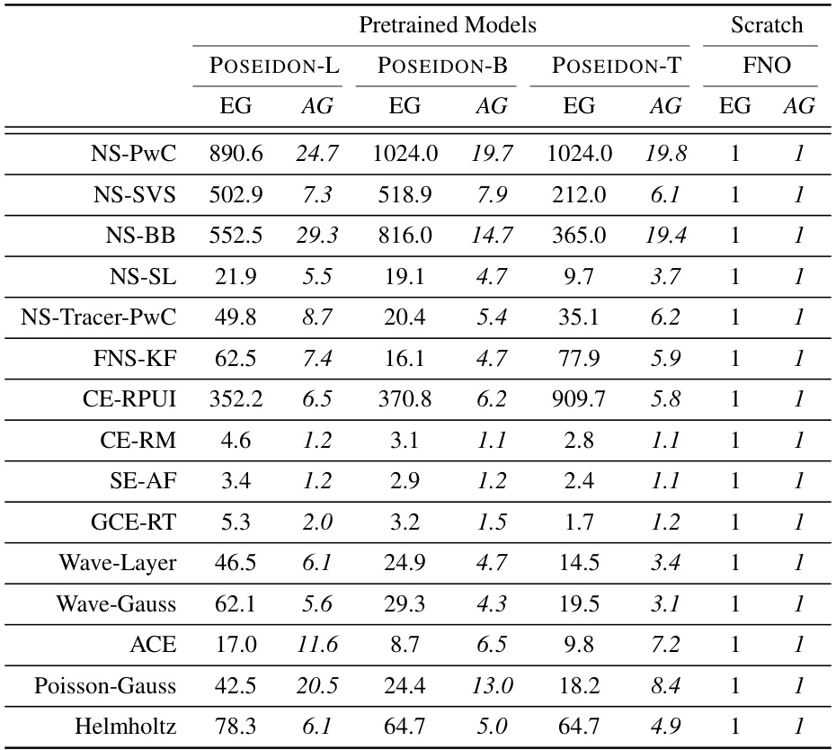
This table presents the efficiency and accuracy gains of various models on different downstream tasks. Efficiency gain (EG) is calculated as the ratio of the number of samples required by FNO to achieve a certain error level to the number of samples required by the model to achieve the same error level. Accuracy gain (AG) is calculated as the ratio of the error achieved by FNO to the error achieved by the model, both using the same number of samples. The table allows a comparison of the relative performance of POSEIDON against other models and across different downstream tasks.
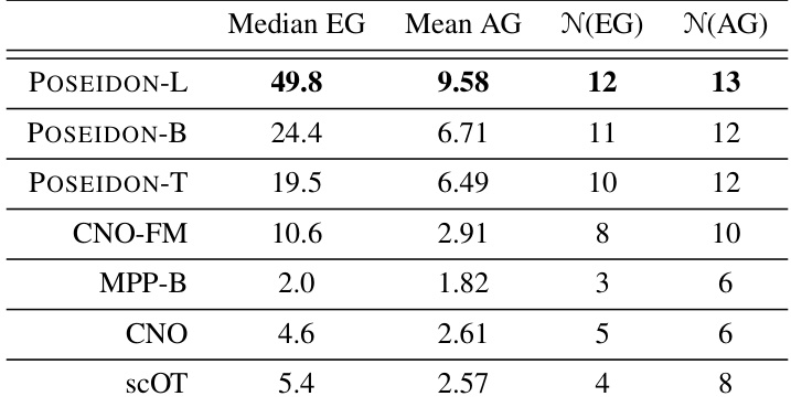
This table summarizes the performance of various models (POSEIDON-L, POSEIDON-B, POSEIDON-T, CNO-FM, MPP-B, CNO, scOT) across all 15 downstream tasks. The median efficiency gain (EG) indicates how many fewer samples a model needs compared to FNO to achieve the same error level. The mean accuracy gain (AG) shows the average accuracy improvement of the model compared to FNO. N(EG) and N(AG) represent the number of tasks where EG and AG exceed certain thresholds (10 and 2, respectively), offering insights into the overall effectiveness of each model.

This table presents the efficiency and accuracy gains of the DPOT model on several downstream tasks. Efficiency gain (EG) is calculated by comparing the number of samples needed by DPOT to achieve a certain error level to the number of samples required by FNO to reach the same error level. Accuracy gain (AG) shows the improvement in accuracy achieved by DPOT over FNO when both models are trained with the same number of samples. Different DPOT configurations (M,L) are tested, and results are shown for both fine-tuned and scratch-trained models.

This table presents the efficiency and accuracy gains of different models (POSEIDON-L, CNO-FM, MPP-B, CNO, scOT, and FNO) across 15 downstream tasks. Efficiency gain (EG) shows how many fewer samples a model needs compared to FNO to achieve the same error level. Accuracy gain (AG) shows the relative accuracy improvement of a model over FNO with a fixed number of samples. The results highlight POSEIDON’s superior performance in both sample efficiency and accuracy.

This table presents the efficiency and accuracy gains of different models compared to the FNO baseline across 15 downstream tasks. Efficiency gain (EG) shows how many fewer samples a model needs to achieve the same error as FNO. Accuracy gain (AG) shows the relative improvement in accuracy for a given number of samples.
Full paper#
