PowerPM: Foundation Model for Power Systems

↗ OpenReview ↗ NeurIPS Homepage ↗ Chat

TL;DR

#

Key Takeaways

#

Why does it matter?

#

This paper is crucial for researchers in power systems because it introduces PowerPM, a foundation model that significantly advances electricity time series (ETS) data modeling. Its off-the-shelf nature and superior performance across diverse tasks make it a valuable tool. Moreover, the study’s novel self-supervised pre-training framework and generalization ability open exciting avenues for future research in this field.

Visual Insights

#

This figure illustrates several key aspects of electricity time series (ETS) data and its applications in power systems. Panel (a) depicts the hierarchical structure of ETS data, starting from the city level and going down to individual users. This hierarchy is important because it allows for different levels of aggregation and analysis. Panel (b) shows the temporal dependencies within an ETS window, which means that data points closer together in time are more likely to be correlated, but exogenous variables (like weather) can also play a role. Panel (c) shows that different instances (e.g., households) may have diverse electricity consumption patterns. Panel (d) shows various tasks related to ETS data analysis, including demand-side management, grid stability, and consumer behavior analysis.

This table presents a comprehensive comparison of the PowerPM model’s performance against various baseline models across a range of downstream tasks within a private dataset. The tasks are categorized into three groups: Demand-side Management, Grid Stability, and Consumer Behavior Analysis. Each task utilizes a specific evaluation metric (MSE for forecasting and imputation, F0.5 for anomaly detection, and Accuracy for classification). The table highlights PowerPM’s superior performance across the board, even when compared to a frozen version of the model (PowerPM freeze).

In-depth insights

#

ETS Foundation Model

#

An ETS Foundation Model is a significant advancement in power systems analysis. By leveraging the abundance of electricity time-series data, it aims to create a general-purpose model capable of handling diverse downstream tasks. This approach tackles the challenges of ETS data’s inherent complexity, including its hierarchical structure and intricate temporal dependencies influenced by exogenous variables. The model’s design likely incorporates sophisticated techniques such as temporal and hierarchical encoders to capture these multifaceted relationships. Self-supervised pre-training is a key component, enabling the model to learn robust representations from unlabeled data. This pre-training likely involves innovative methods to handle temporal dependencies within and across ETS windows. The expectation is that this foundation model will significantly improve the performance of various power systems applications, and it is anticipated to be adaptable and generalizable across different domains and tasks, demonstrating significant improvements in performance compared to existing specialized models.

Hierarchical Encoding

#

Hierarchical encoding in the context of electricity time series (ETS) modeling is a crucial technique for capturing the complex, multi-level relationships inherent in the data. Power systems data naturally exhibits a hierarchical structure, ranging from individual consumers to districts, cities, and entire grids. A hierarchical encoder, therefore, must effectively integrate information across these various granularities to provide a comprehensive understanding of power consumption patterns. This is achieved by modeling correlations between different levels of the hierarchy, allowing the model to learn both macro-level trends (e.g., city-wide consumption) and micro-level details (e.g., individual user behavior). This multi-scale approach is particularly beneficial for tasks that require an understanding of the interplay between different levels of the system, such as demand-side management, where understanding individual consumer behavior is as important as overall grid stability. The effectiveness of hierarchical encoding relies on the choice of architecture; graph neural networks (GNNs) are particularly well-suited for this task due to their ability to naturally represent and process hierarchical relationships within a graph structure. The success of this method is also critically dependent on the design of the pre-training strategy, as it needs to effectively learn the hierarchical dependencies for improved performance on downstream tasks. Therefore, a robust pre-training framework is essential for successful implementation of a hierarchical encoder.

Self-Supervised Learning

#

Self-supervised learning (SSL) is a powerful technique that allows models to learn from unlabeled data by creating pretext tasks. In the context of time series analysis, like that concerning power systems, this is particularly valuable given the abundance of readily available unlabeled electricity time series data. PowerPM leverages SSL by employing masked time series modeling and dual-view contrastive learning. Masked modeling forces the model to reconstruct missing portions of a time series, improving its understanding of temporal dependencies. Contrastive learning encourages the model to learn a robust representation by comparing similar time series windows from the same instance (positive pairs) and contrasting them with dissimilar ones from different instances or time windows (negative pairs). This dual-view approach, considering temporal and instance perspectives, enriches the model’s understanding of both short-term dynamics and broader patterns across various time scales and instances. The effectiveness of this dual-pronged SSL approach is demonstrated in PowerPM’s superior performance compared to purely supervised models, highlighting the significance of SSL for effectively utilizing vast quantities of unlabeled data in power system applications. The self-supervised pre-training step significantly boosts performance on downstream tasks, showcasing the power of SSL for model generalization across diverse power system scenarios.

PowerPM Generalization

#

The PowerPM model’s generalization capabilities are a crucial aspect of its effectiveness as a foundation model for power systems. Strong generalization implies the model’s ability to perform well on unseen data and diverse downstream tasks beyond the specific datasets used during pre-training. The paper likely evaluates generalization by testing PowerPM’s performance on various public datasets, distinct from its private pre-training data. Success in this evaluation would demonstrate the model’s ability to transfer knowledge acquired during pre-training to new domains, showcasing robustness and adaptability. Key aspects to analyze within the context of generalization would include the performance consistency across different tasks and datasets, the model’s resilience to data variations (noise, missing values), and its sensitivity to different data granularities or hierarchical levels inherent in power systems. Quantifiable metrics such as accuracy, mean squared error, and F1-score, across these diverse scenarios, would be critical for assessing the extent of PowerPM’s generalization strength. A thorough analysis would likely include comparison with other state-of-the-art models to benchmark its generalization ability.

Future Work

#

Future research directions stemming from this PowerPM foundation model could involve several key areas. Extending the model’s capabilities to encompass a wider range of power system data types beyond electricity time series (ETS) is crucial. This could include incorporating data from smart meters, grid sensors, and renewable energy sources to create a more holistic representation of the power grid. Another important direction would be improving the model’s scalability and efficiency. The current model, while powerful, has a significant parameter count. Investigating model compression techniques or exploring alternative architectural designs to reduce the computational burden without sacrificing performance is vital for wider adoption. Finally, enhanced interpretability should be prioritized. While the model demonstrates strong performance, understanding its internal decision-making processes is essential for building trust and ensuring responsible deployment. This necessitates further research into explainable AI (XAI) techniques tailored to the power systems domain. Addressing fairness and bias within the model’s predictions is another critical area requiring attention. This could involve developing methods to detect and mitigate potential biases arising from inherent imbalances in the training data. Further work should explore the potential of PowerPM to facilitate new applications in the power systems sector, including predictive maintenance, anomaly detection, and grid modernization planning. The model’s remarkable generalization ability suggests a broad range of promising applications that merit further investigation.

More visual insights

#

More on figures

This figure compares the performance of PowerPM against several baseline models across various downstream tasks categorized into three groups: Demand-side Management, Grid Stability, and Consumer Behavior Analysis. Each group is represented by a radar chart showing the relative performance of each model on a set of specific tasks. This visualization provides a comprehensive overview of PowerPM’s performance compared to other state-of-the-art methods across diverse tasks relevant to power systems.

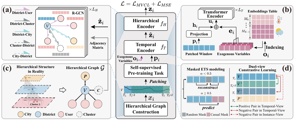
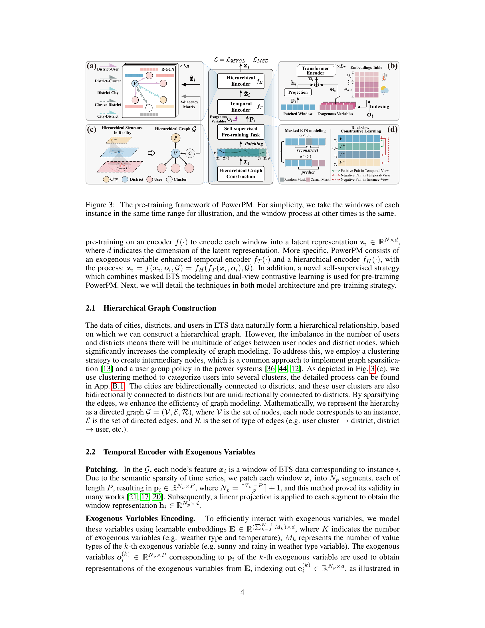
This figure illustrates the pre-training framework of the PowerPM model. It shows the process of constructing a hierarchical graph from the ETS data, using a temporal encoder to capture temporal dependencies and incorporate exogenous variables, and employing a hierarchical encoder to model correlations between different levels of the hierarchy. The self-supervised pre-training strategy, which combines masked ETS modeling and dual-view contrastive learning, is also depicted. The figure breaks down the process into stages, showing the input data, the temporal and hierarchical encoding processes, the masked ETS modeling, and the dual-view contrastive learning, ultimately producing a latent representation for each ETS window.

This figure illustrates the pre-training framework of the PowerPM model. It shows the hierarchical graph construction, the temporal encoder with exogenous variables, and the self-supervised pre-training task, which includes masked ETS modeling and dual-view contrastive learning. The temporal encoder uses a Transformer to capture temporal dependencies, incorporating exogenous variables. The hierarchical encoder uses R-GCN to model correlations between different hierarchical levels. The self-supervised learning framework aims to improve the model’s understanding of both temporal dependencies within ETS windows and the discrepancies across different windows. This comprehensive framework enables PowerPM to learn a robust and generalizable representation for various downstream tasks.

More on tables

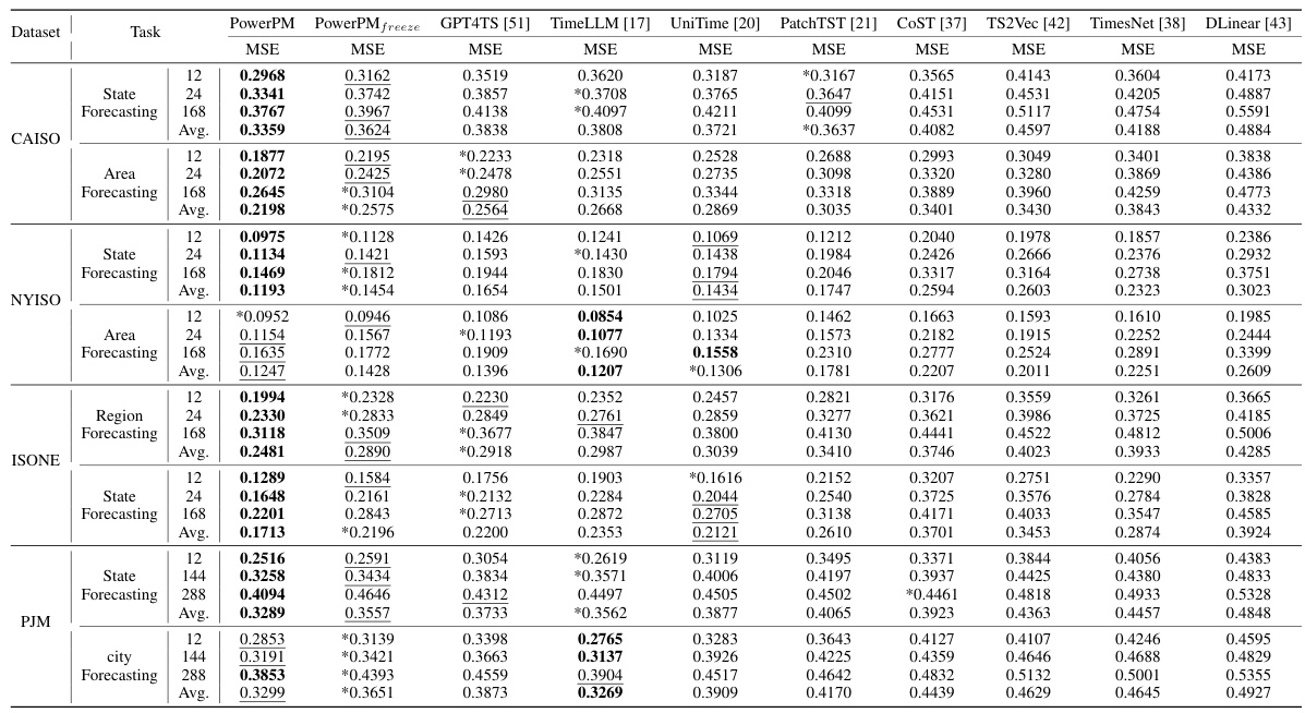
This table presents a comparison of the performance of PowerPM and several baseline models on four different public datasets. The performance is evaluated across various forecasting tasks with different prediction horizons. The datasets represent different geographic locations and hierarchical structures, allowing for an assessment of PowerPM’s generalization ability. The metrics used are MSE (Mean Squared Error).

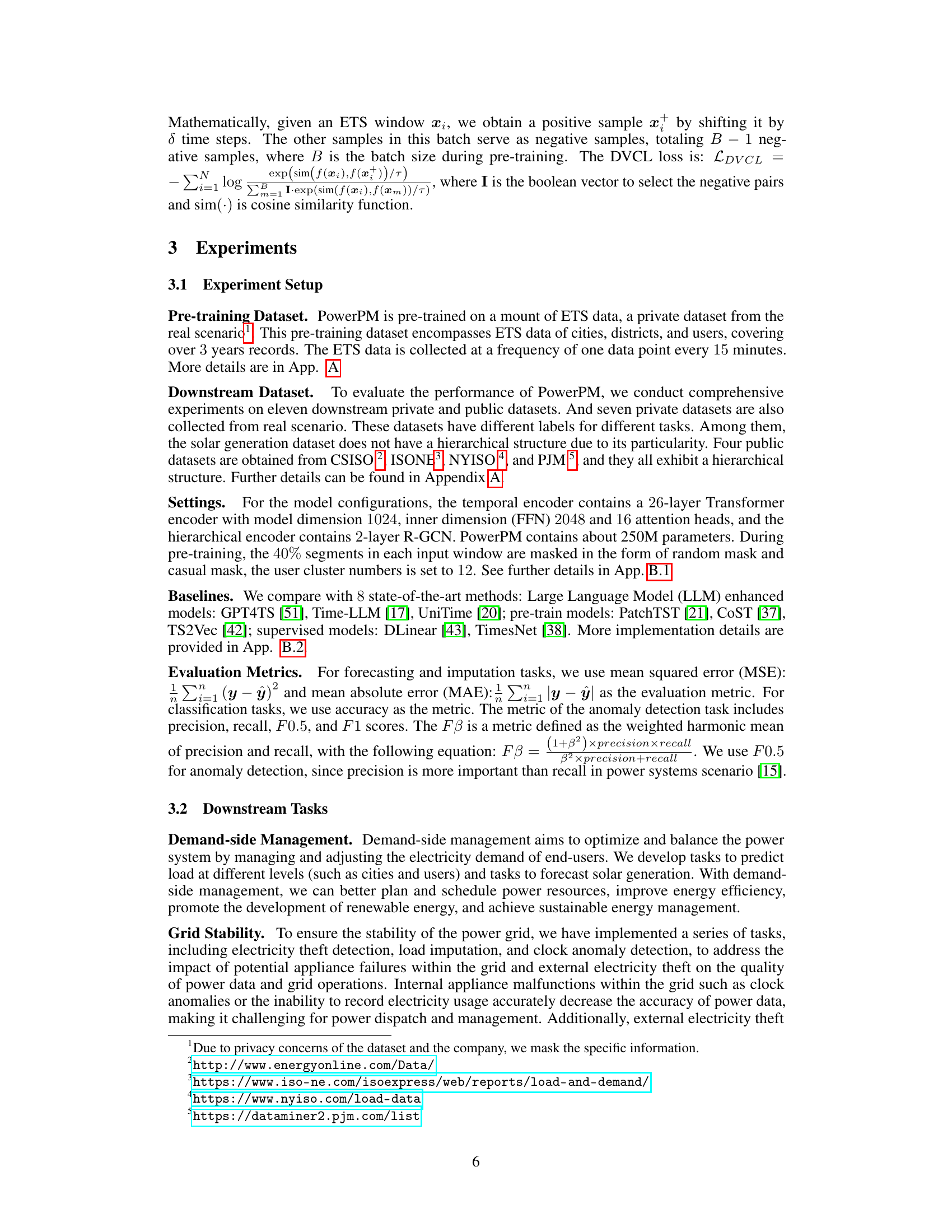
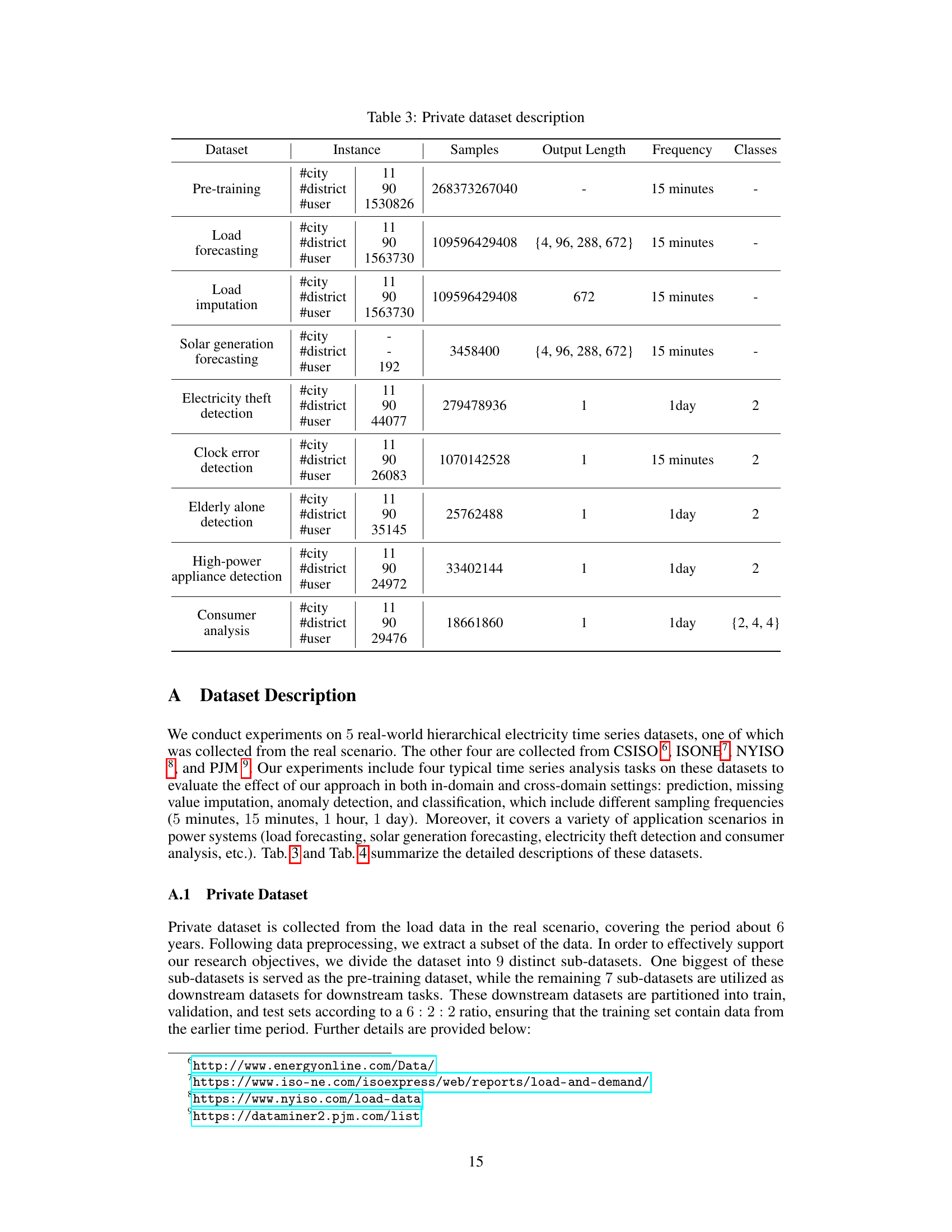
This table provides detailed information about the private datasets used in the research. It lists the dataset type, the number of cities, districts, and users included, the total number of samples, the length of each output sequence (in terms of time points), the data recording frequency, and the number of classes or categories present in the data. Each row represents a specific dataset used for a specific task within the study, such as pre-training, load forecasting, or anomaly detection. The information in this table is crucial to understanding the scale and characteristics of the datasets used in the PowerPM model experiments.

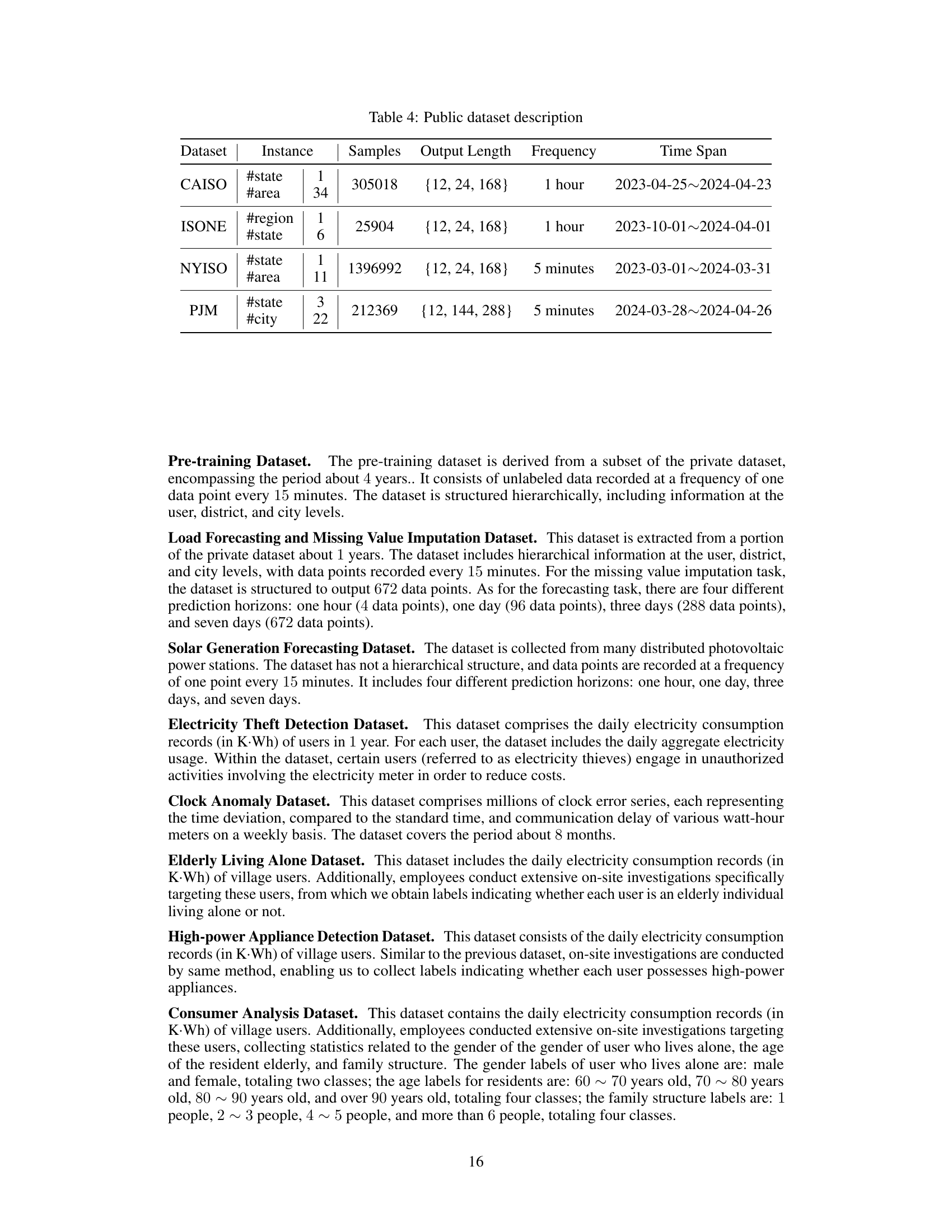
This table presents a summary of the four public datasets used in the paper’s experiments. For each dataset (CAISO, ISONE, NYISO, PJM), it lists the instance type (#state, #area, #region, #city), the number of samples, the output lengths (time horizons for forecasting tasks), the data frequency (how often data points are recorded), and the overall time span covered by the data.

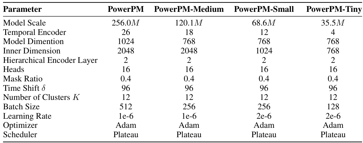
This table shows the different hyperparameters used for training four different size variants of the PowerPM model. It details the configuration for the temporal and hierarchical encoders, including the number of layers, dimensions, heads, mask ratio, time shift, number of clusters, batch size, learning rate, optimizer, and scheduler. These specifications highlight how model size influences training parameters.

This table presents a detailed performance comparison using the Mean Absolute Error (MAE) metric on a private dataset. It breaks down the results for different forecasting horizons (4, 96, 288, and 672 time points) and varying data imputation mask ratios (0.125, 0.25, 0.375, and 0.5). The input window size used for all tasks was 672. The comparison includes PowerPM and its variants, along with several other baseline models.

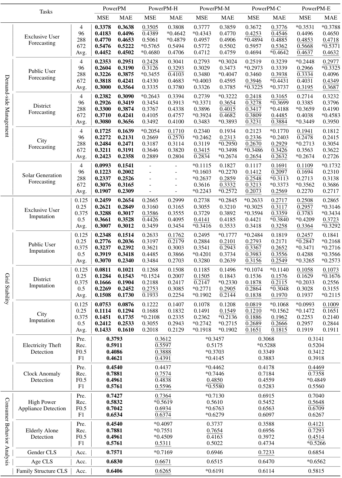
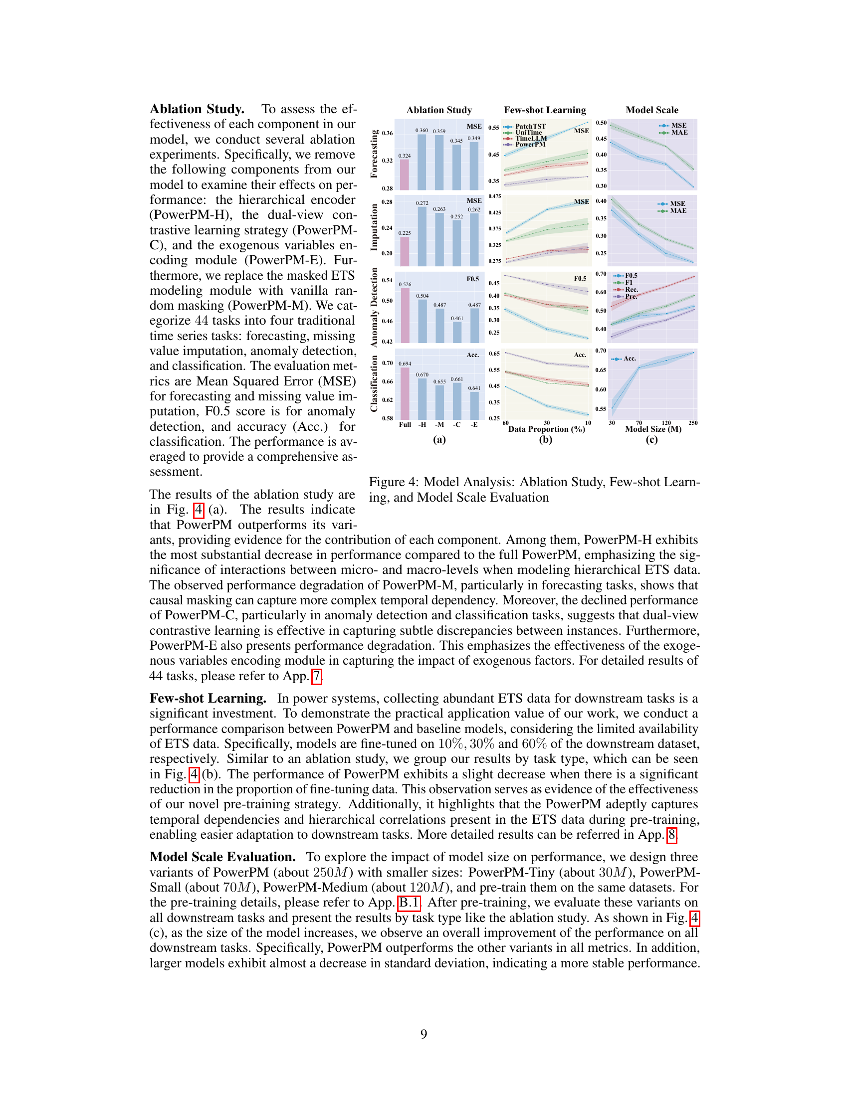
This table presents the results of ablation studies conducted to evaluate the impact of each component in the PowerPM model. The model’s performance across various downstream tasks (forecasting, imputation, anomaly detection, and classification) is compared across several ablation variants. Each variant excludes one component of the model (hierarchical encoder, dual-view contrastive learning, exogenous variables encoding, or the masked ETS modeling module). The results show the relative importance of each component in achieving the overall model’s performance. The table displays the mean squared error (MSE) and mean absolute error (MAE) for forecasting and imputation tasks, the F0.5 score for anomaly detection, and the accuracy (Acc.) for classification tasks.

This table presents a comprehensive comparison of the performance of various models in a few-shot learning scenario. The models are evaluated on forecasting, imputation, anomaly detection, and classification tasks using different proportions of the downstream dataset (10%, 30%, 60%). The performance metrics used are MSE for forecasting and imputation, F0.5 for anomaly detection, and accuracy for classification. Different time horizons are considered for forecasting.

Full paper

#