↗ OpenReview ↗ NeurIPS Homepage ↗ Chat
TL;DR#
Analyzing inter-individual variability in physiological time series is challenging due to irregularities in sampling and variations in length. Existing unsupervised representation learning methods often struggle with these complexities, leading to suboptimal feature extraction and reduced interpretability. Shape analysis offers a potential solution, but generalizing it to time series with varied structures is difficult.
This paper proposes TS-LDDMM, a novel unsupervised method that addresses these issues. TS-LDDMM represents time series as deformations of a reference series, using diffeomorphisms to learn shape-based features. The algorithm excels at handling irregularities and provides interpretable results, outperforming state-of-the-art methods in real-world and synthetic datasets. It is backed by a representation theorem providing a solid theoretical foundation.
Key Takeaways#
Why does it matter?#
This paper is crucial for researchers working with time-series data, particularly in biomedical applications. It introduces a novel unsupervised method (TS-LDDMM) that effectively handles the complexities of irregularly sampled, multi-variate time series. The shape-based representation learned by TS-LDDMM offers enhanced interpretability, surpassing existing methods in several benchmarks. This opens exciting avenues for further research in diverse fields needing advanced time-series analysis.
Visual Insights#
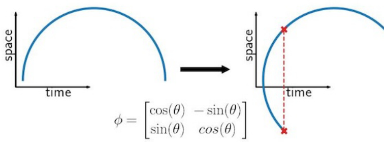
The figure illustrates how applying a general diffeomorphism to a time series graph can distort the time series structure. A general diffeomorphism, which is a transformation that maps a space onto itself in a smooth, invertible way, can map a single time point to multiple spatial points, thus losing the original time series’ structure and making it inappropriate for analysis.

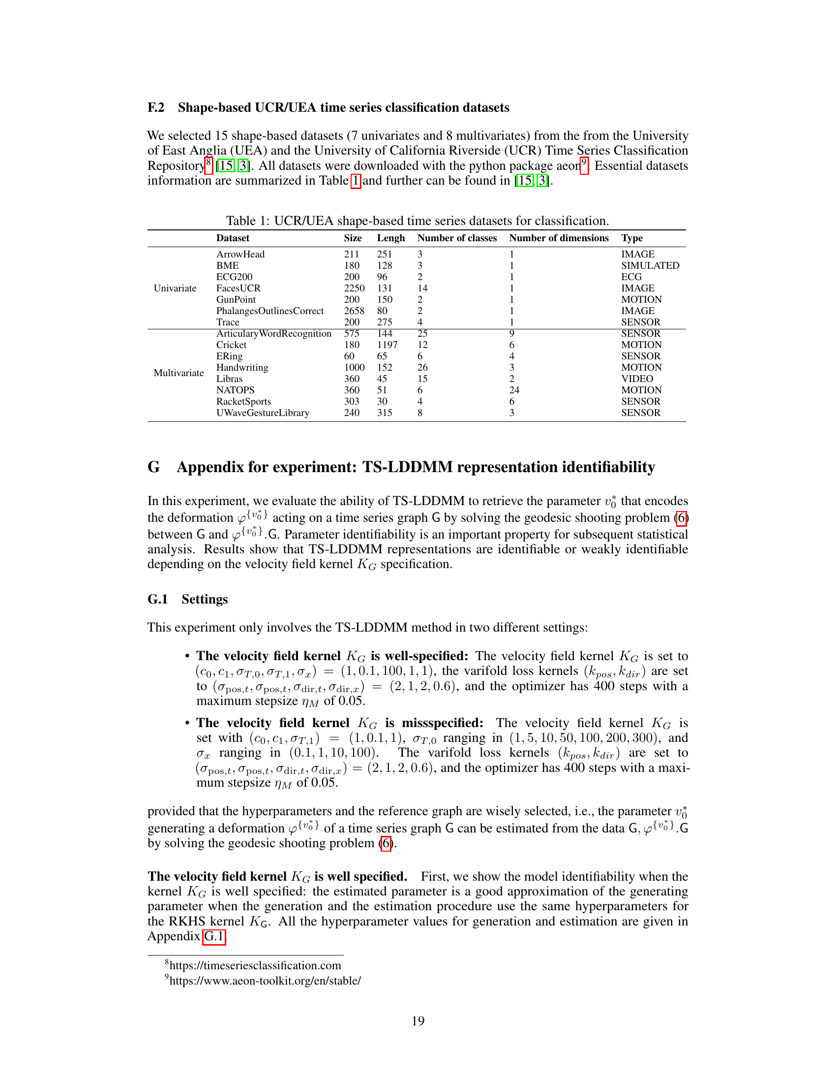
This table lists fifteen datasets used in the paper’s experiments to evaluate the performance of TS-LDDMM and other methods on shape-based time series classification tasks. Each dataset is characterized by its size (number of instances), length (number of time points), number of classes, number of dimensions (univariate or multivariate), and the type of data it represents. This information is crucial for understanding the context and scope of the experimental evaluations presented in the paper.
In-depth insights#
TS-LDDMM Method#
The TS-LDDMM method, a novel unsupervised approach for analyzing inter-individual variability in time series data, presents a significant advancement in the field. Its core innovation lies in representing time series as deformations of a reference series, leveraging the power of Large Deformation Diffeomorphic Metric Mapping (LDDMM). Unlike traditional methods, TS-LDDMM explicitly addresses the unique structure of time series graphs, ensuring that transformations maintain temporal coherence. This results in shape-based representations that are both robust to irregularities in sampling and highly interpretable, opening doors for downstream analysis in various biomedical applications. By establishing a representation theorem for time series graphs and integrating it within the LDDMM framework, TS-LDDMM provides a theoretically grounded and practically effective method. The use of synthetic and real-world data demonstrates its capacity to handle irregularly sampled, multivariate time series, showcasing advantages over existing approaches in both accuracy and interpretability. The method’s ability to extract meaningful features from complex temporal data makes it a promising tool for diverse applications requiring the analysis of inter-individual variations.
Shape Representation#
The concept of ‘Shape Representation’ in time series analysis is crucial for capturing the underlying patterns and variability within the data. Effective shape representation methods should handle irregularities in sampling, variable lengths, and multivariate data. The choice of representation significantly impacts the downstream analysis, whether it is classification, clustering, or anomaly detection. A strong shape representation should be robust to noise and distortions, while preserving essential information about the temporal dynamics. For example, representing time series as deformations of a reference series, as done in the TS-LDDMM method, offers a powerful approach for capturing inter-individual variability in physiological data. However, the choice of diffeomorphism and distance metric play a crucial role. Alternatives like Shape-FPCA use functional data analysis techniques, often requiring interpolation or smoothing, which may affect the shape details. Ultimately, the optimal approach depends on the specific application and dataset characteristics; the key is in choosing a representation that balances the need for information preservation with computational tractability and interpretability.
Irregular Sampling#
Irregular sampling in time series data presents significant challenges for analysis. Traditional methods often assume evenly spaced data points, making them unsuitable for datasets with missing or irregularly timed observations. Handling missing data is crucial, as simply discarding incomplete records can lead to biased results and loss of valuable information. Imputation techniques, such as linear interpolation or more sophisticated statistical methods, can help to fill in missing values, but they introduce uncertainty and can distort the underlying patterns. Advanced techniques, like those based on flexible modeling frameworks (e.g., functional data analysis), provide more robust approaches, capable of handling both irregular sampling and variability in time series lengths. These methods offer improved accuracy and reliability compared to simpler methods but may increase computational complexity. The choice of method depends on the nature of the data, the goals of the analysis, and the acceptable trade-off between accuracy and computational cost. Careful consideration of the implications of missing data and the choice of appropriate analytical methods are essential for obtaining reliable results.
Biomedical App.#
The heading ‘Biomedical App.’ suggests a section detailing the applications of the research within the biomedical field. A thoughtful analysis would expect this section to showcase the practical utility of the presented methods. It likely involves real-world examples demonstrating how the algorithms or techniques effectively address specific biomedical problems. The examples could range from analyzing physiological signals (ECG, EEG) to identifying patterns in medical images, potentially highlighting improved diagnostic accuracy, better treatment planning, or new insights into disease mechanisms. A strong presentation would demonstrate the advantages over existing methods, addressing issues like scalability, interpretability, and the handling of complex, noisy data, often encountered in real biomedical datasets. Finally, a discussion of potential limitations and future directions of the research in the biomedical context should conclude this section, thereby establishing its relevance and impact.
Future Research#
Future research directions stemming from this work could explore several promising avenues. Extending TS-LDDMM to handle even higher-dimensional time series data, such as video or multi-modal physiological signals, would significantly broaden its applicability. Further investigation into more sophisticated loss functions that are robust to noise and irregular sampling, potentially leveraging recent advances in deep learning, is warranted. Developing adaptive methods for hyperparameter tuning would improve user-friendliness and reduce the computational burden. Finally, a critical area for future work is rigorous evaluation on larger, more diverse datasets, especially in the context of real-world clinical applications, to assess the generalizability and practical impact of this shape-based representation learning approach. The potential for improved interpretability through visualization techniques and qualitative analysis of learned deformations also merits further attention.
More visual insights#
More on figures

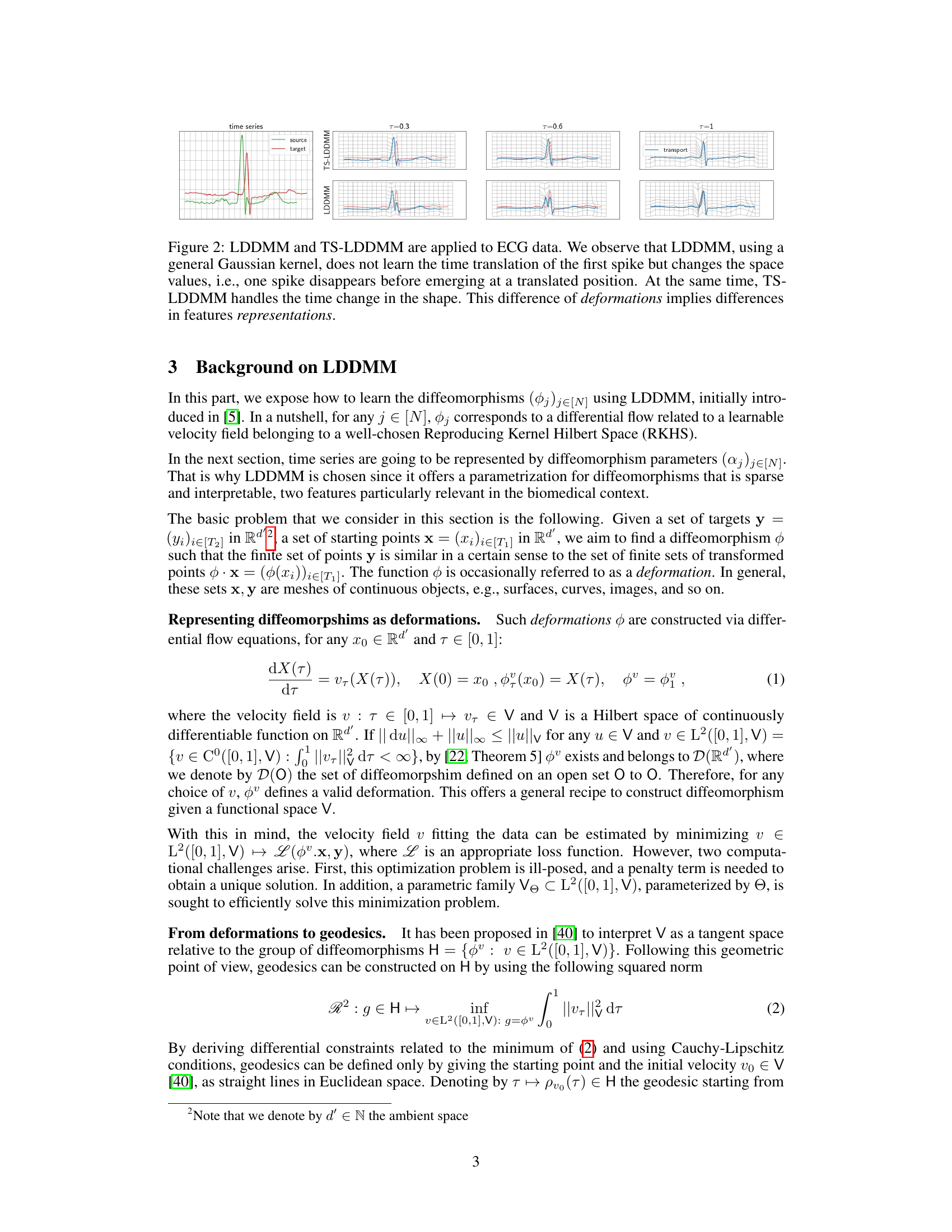
This figure compares the performance of LDDMM and TS-LDDMM on ECG data. LDDMM, using a general Gaussian kernel, fails to accurately capture the time translation of a key feature (spike), instead altering its spatial representation. TS-LDDMM, however, successfully models the time translation, preserving the shape’s temporal integrity. This difference in how the two methods handle deformations highlights the key advantage of TS-LDDMM in learning time-aware shape representations.

This figure compares the principal component analysis (PCA) results obtained using TS-LDDMM and LDDMM for analyzing mice ventilation before drug exposure. The left plots in (a) and (b) show the distribution of the principal components (PC1 and PC2) according to the mouse genotype (ColQ or WT). The right plots illustrate the deformations of a reference respiratory cycle along the PC axes, offering insights into the types of shape variations captured by each method. The comparison aims to highlight differences in how TS-LDDMM and LDDMM represent and analyze respiratory cycles.

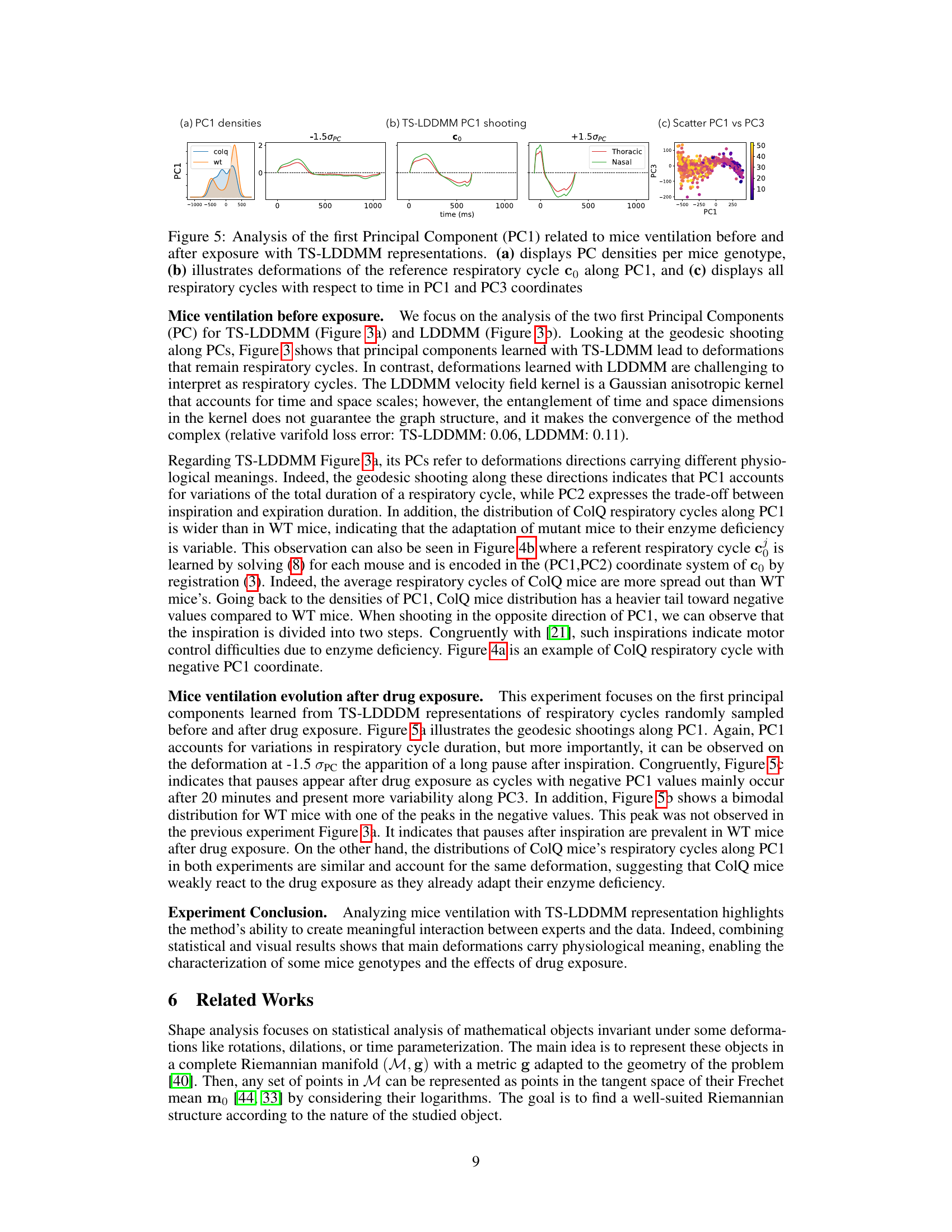
This figure shows the analysis of the first principal component (PC1) of mice ventilation data before and after drug exposure using TS-LDDMM. Panel (a) presents the distribution of PC1 values for control (WT) and mutant (ColQ) mice. Panel (b) illustrates how the reference respiratory cycle is deformed along PC1. Panel (c) shows a scatter plot of PC1 versus PC3, visualizing the respiratory cycles in this two-dimensional PC space.

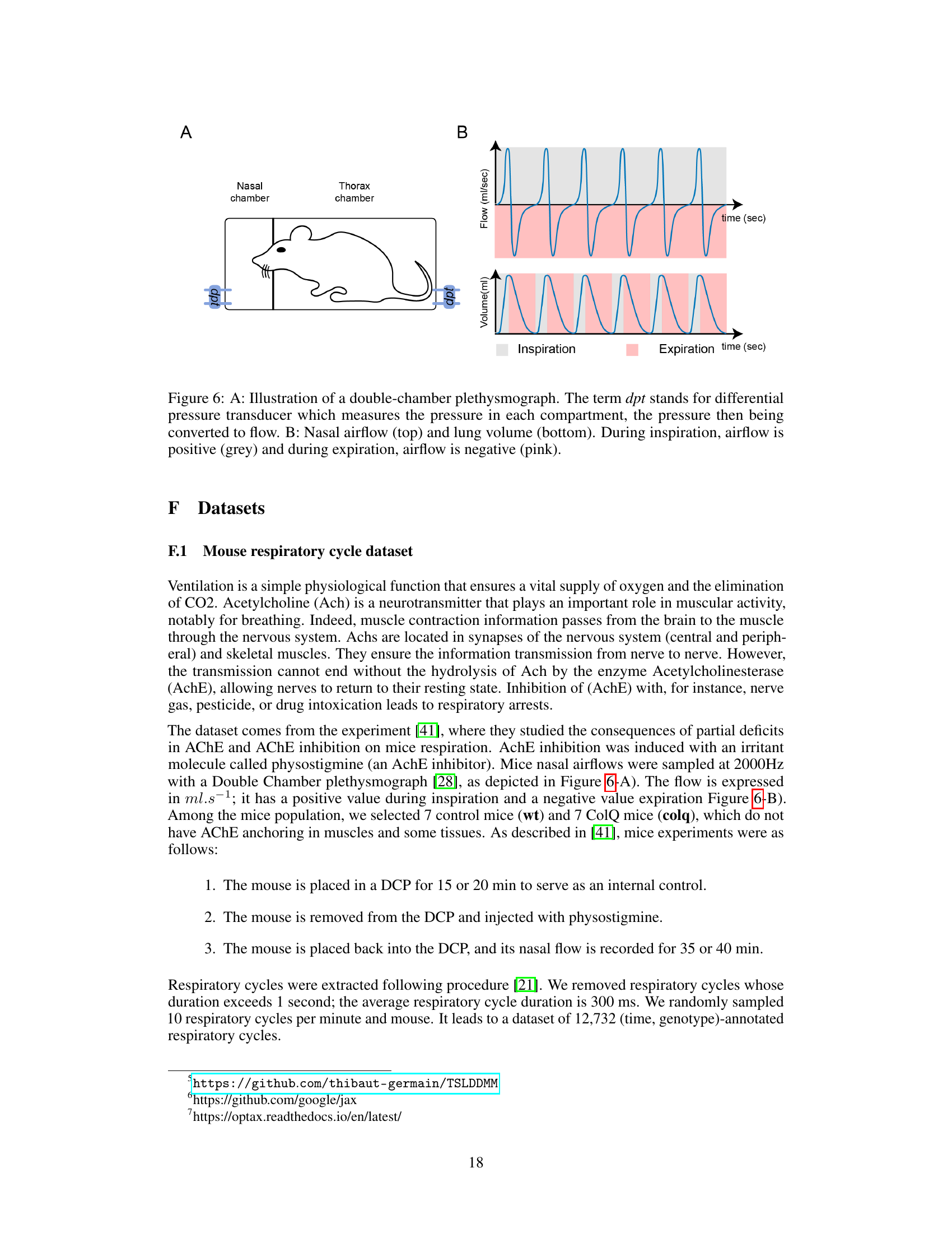
This figure shows a schematic of a double-chamber plethysmograph used to measure respiratory airflow and volume in mice. Panel A illustrates the setup: a mouse is placed in a chamber divided into two compartments, one for the nose and one for the thorax. Differential pressure transducers (dpt) measure the pressure difference between these compartments which is then converted to calculate airflow. Panel B depicts example recordings of nasal airflow (upper graph) and lung volume (lower graph). Positive values for airflow denote inspiration, and negative values denote expiration. The shading indicates the phases of the respiratory cycle.

This figure shows the results of applying a diffeomorphism (a transformation of the graph of a time series) parametrized by a* to a reference time series graph. Three different sets of parameters (ta, sa, ms) were used, resulting in three different transformed time series. The original time series (reference s0) is also plotted for comparison. The plot illustrates how changes in the sampling parameters of a* affect the shape of the transformed time series, demonstrating the sensitivity of the method to these parameters. This is relevant to understanding how well the model can reconstruct a time series from its graph using different parameterizations. The x-axis represents time, and the y-axis represents the value of the time series.
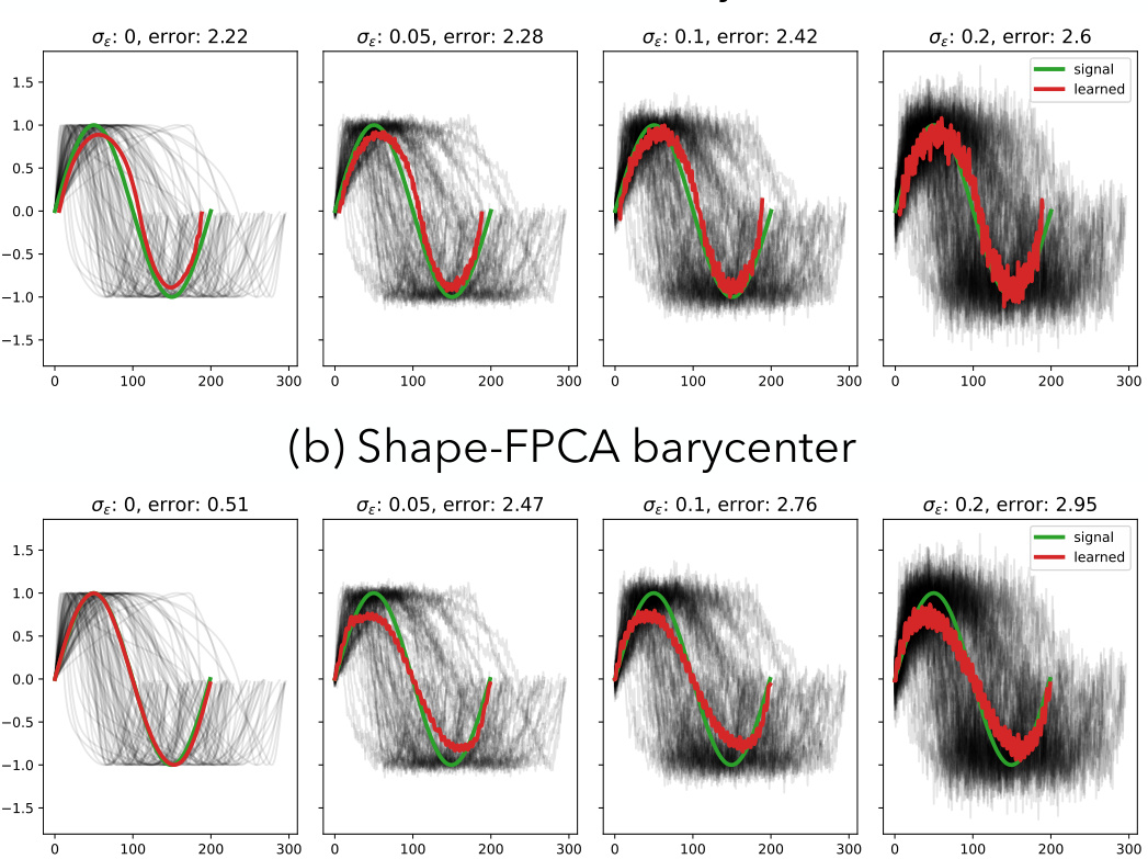
This figure compares the performance of TS-LDDMM and Shape-FPCA in learning the barycenter of a set of noisy sine waves. The top row shows the results for TS-LDDMM, while the bottom row shows the results for Shape-FPCA. The green line represents the true barycenter (mean), while the red line is the learned barycenter. The gray lines represent the individual noisy sine waves. The error values are reported in the title of each subplot. The figure demonstrates that both methods are sensitive to noise, but TS-LDDMM is more robust and maintains a better approximation of the true barycenter even at higher noise levels.

This figure shows the results of applying TS-LDDMM to analyze mice ventilation data before and after drug exposure. Panel (a) shows the distribution of the first principal component (PC1) for control and ColQ mice. PC1 appears to represent the duration of the respiratory cycle. Panel (b) shows how the reference respiratory cycle is deformed along PC1, illustrating the changes in the shape of the respiratory cycle. Panel (c) displays all respiratory cycles projected onto the PC1 and PC3 axes.

This figure compares the results of applying TS-LDDMM and LDDMM to analyze mice ventilation data before drug exposure. The left plots in (a) and (b) show the density of the principal components (PCs) for each genotype (ColQ and WT). The right plots display the deformations of a reference respiratory cycle along the principal component axes. The comparison highlights the difference in the type of deformations captured by the two methods. TS-LDDMM learns deformations that maintain the structure of respiratory cycles, while LDDMM produces less interpretable changes.
More on tables
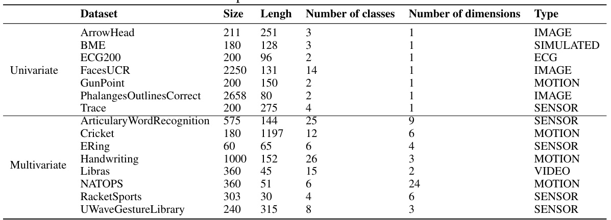
This table lists 15 datasets used in the paper’s experiments. Each row represents a single dataset and provides information crucial for understanding the data used in the experiments. This includes the dataset name, its size (number of time series), the length of each time series, the number of classes within the dataset, the number of dimensions or variables per time series, and the type of data (e.g., image, motion, sensor). The datasets are categorized as either univariate (one variable per time series) or multivariate (multiple variables per time series). This table is vital to understanding the scope and nature of the experiments conducted in the paper, ensuring reproducibility and comparability with other research using the same datasets.

This table presents the results of the loss function L between the true transformation of the graph of the time series and the estimated transformation. The loss is computed for different values of the sampling parameters, and for different values of the hyperparameters of the kernel KG. The results show the impact of the hyperparameters on the accuracy of the estimation.

This table presents the results of comparing TS-LDDMM with other methods on 15 datasets under four different sampling regimes (0%, 30%, 50%, and 70% missing rates). The comparison is based on the average macro F1-score and rank of the methods. TS-LDDMM shows to be the best performing method across three out of the four sampling regimes.

This table lists 15 datasets used in the paper’s experiments for evaluating the performance of the proposed TS-LDDMM method and comparing it to other methods. Each dataset’s name, size, length of time series, number of classes, number of dimensions, and data type are provided. The datasets are categorized into univariate and multivariate for easy reference. This allows readers to understand the characteristics of the datasets used for the classification task and compare the results across different data characteristics.
Full paper#


