↗ OpenReview ↗ NeurIPS Homepage ↗ Chat
TL;DR#
Many machine learning models deployed in real-world applications struggle with changes in data distribution (distribution shifts), particularly when these shifts negatively impact model performance. Existing methods for detecting these harmful shifts often require access to labeled data, which is usually unavailable in production settings, thus making them impractical. This creates a significant challenge for ensuring the reliability and safety of deployed AI systems.
This paper presents a novel approach to tackle this problem. It introduces a label-free method that uses a proxy for true model error (derived from a secondary error estimation model) and a sequential statistical test to monitor changes in the error rate over time. The method effectively balances the detection power and false alarm rate while not needing to explicitly access labels in production, a significant improvement over the current state-of-the-art solutions. The experimental findings demonstrate the method’s effectiveness across various types of distribution shifts and diverse datasets.
Key Takeaways#
Why does it matter?#
This paper is crucial for researchers working on robust AI systems and model monitoring. It addresses the critical need for detecting harmful distribution shifts in real-world applications without relying on labels, a significant limitation of existing methods. The proposed approach offers improved practicality and broad applicability across diverse domains. This opens new avenues for research in unsupervised anomaly detection, sequential changepoint analysis, and the development of more reliable and safer AI systems.
Visual Insights#
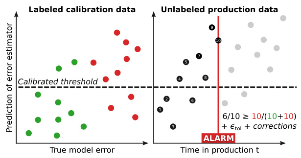
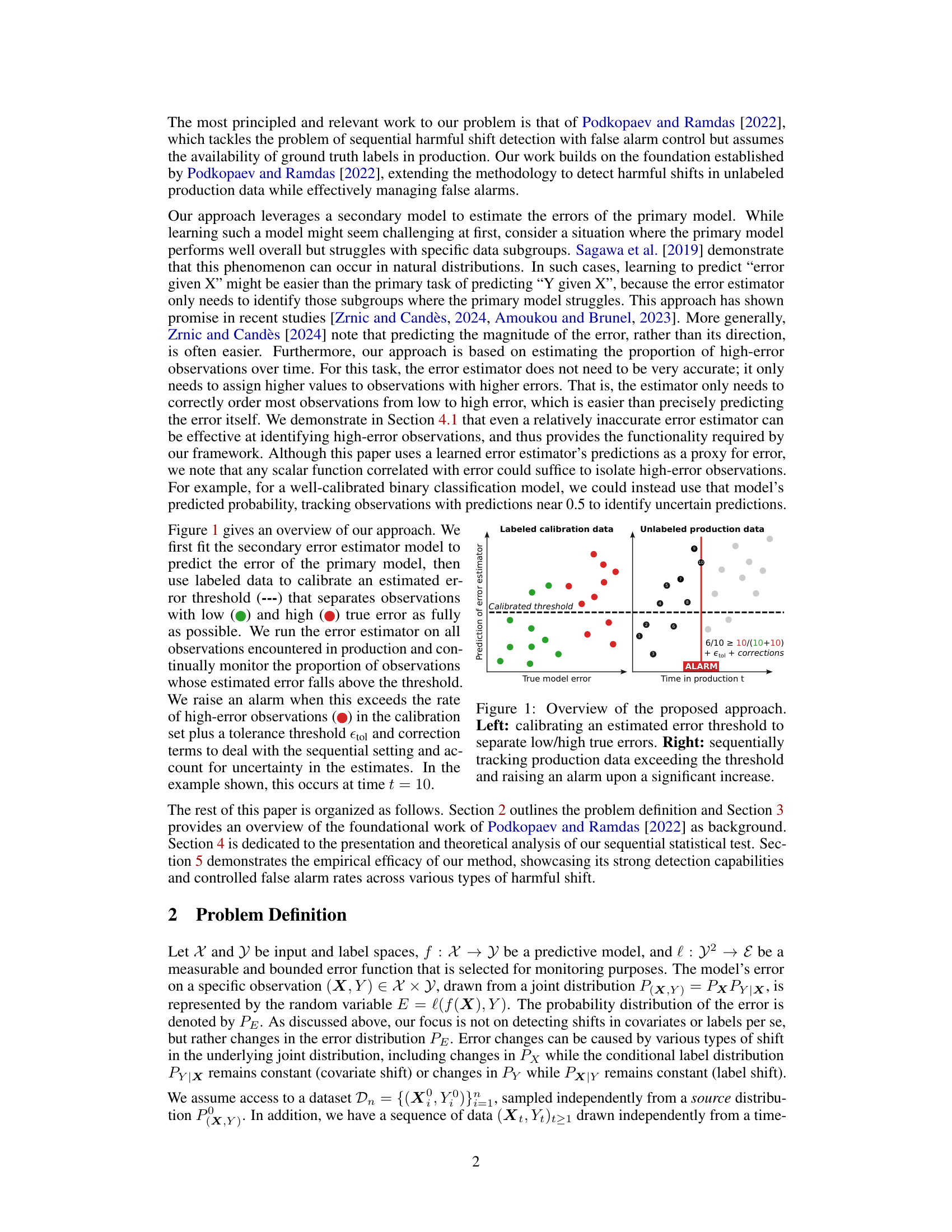
This figure illustrates the two-stage process of the proposed approach for detecting harmful distribution shifts. The left panel shows the calibration stage, where a secondary error estimator model is used with labeled data to establish a threshold that effectively separates observations with low and high true errors. The right panel depicts the online monitoring stage. In this stage, the error estimator is applied to unlabeled production data, and the proportion of observations exceeding the calibrated threshold is continuously tracked. An alarm is triggered when this proportion significantly increases beyond what is expected under the null hypothesis of no harmful shift.
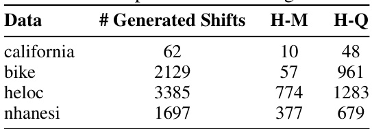
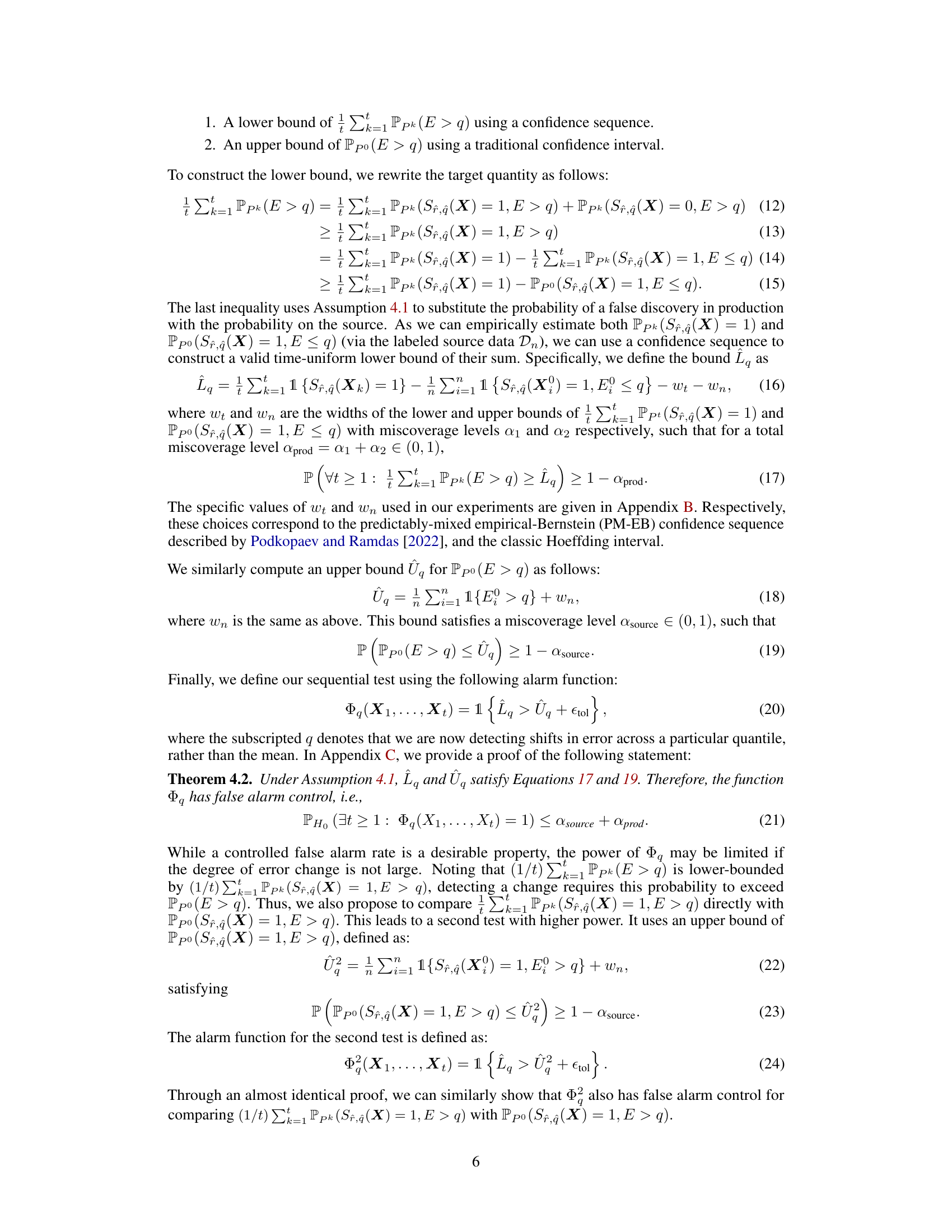
This table shows the number of generated distribution shifts for each dataset (california, bike, heloc, nhanesi) and the number of those shifts detected as harmful by the mean and quantile detectors using the true errors. The ‘H-M’ column indicates the number of harmful shifts detected by the mean detector, while the ‘H-Q’ column represents the number detected by the quantile detector. The data shows that the quantile detector identifies a considerably larger number of harmful shifts than the mean detector across all datasets.
In-depth insights#
Label-Free Shift Detection#
Label-free shift detection addresses a critical challenge in deploying machine learning models: identifying harmful data distribution changes in production environments where obtaining ground truth labels is impractical or impossible. Existing methods often rely on labels, limiting their applicability in real-world scenarios. This label-free approach is crucial because not all distribution shifts are detrimental; some are benign. Therefore, a method to distinguish between harmful and innocuous changes is needed. A promising strategy involves using a secondary model to estimate the primary model’s error, creating a proxy for true error without labels. This error proxy can then be used within a statistical framework to monitor for significant error increases, triggering alerts to indicate harmful shifts. The challenge lies in ensuring that the error estimation model is sufficiently accurate while simultaneously controlling for false positives. Calibration techniques to distinguish between high- and low-error predictions are vital to this process. This approach leverages sequential testing to detect shifts over time, enabling early intervention. The efficacy of this method hinges on the quality of the error estimator and the careful calibration of decision thresholds to effectively balance the detection power and minimize false alarms.
Sequential Error Tracking#
Sequential error tracking in machine learning models deployed in production environments is crucial for detecting harmful distribution shifts. This involves continuously monitoring model performance, not just by evaluating overall accuracy, but by tracking errors over time. A key challenge is handling the absence of ground truth labels in real-world production settings. Effective methods leverage techniques like error estimators or proxies, trained on labeled data, to estimate errors on unlabeled production data. These estimations are then used within a statistical framework, often employing confidence sequences, to detect significant changes in error rates while controlling for false alarms. A significant advantage is the ability to identify harmful shifts early in the production process, enabling timely intervention and preventing significant performance degradation. Sequential analysis is vital in this context, as it provides a principled approach to deal with the accumulation of data over time and the detection of gradual or sudden shifts.
Quantile-Based Approach#
A quantile-based approach offers a robust alternative to traditional mean-based methods for detecting harmful distribution shifts in machine learning models, particularly when dealing with noisy or unreliable error estimations. Instead of focusing on the average error, it tracks the proportion of observations exceeding a specific error quantile. This is particularly advantageous because it is less sensitive to outliers and individual high-error instances that might skew mean-based metrics. The approach leverages the ordinal relationship between observations, requiring only that the error estimator correctly ranks errors rather than accurately predicting their magnitudes. This makes it more reliable when dealing with imperfect error estimators, which is often the case in practice. Calibration of the error threshold is crucial to ensure a desired false positive rate, and a sequential testing framework allows for real-time monitoring of harmful shifts. This methodology demonstrates an effective way to improve performance in situations with limited access to ground truth data and noisy error estimations.
Calibration Methodology#
A robust calibration methodology is crucial for reliable harmful shift detection, especially when dealing with unlabeled production data. The core idea is to train a secondary model that estimates the primary model’s error. This error estimation doesn’t need perfect accuracy; rather, it needs to effectively rank observations by their error magnitudes. A calibration step then identifies an optimal threshold, separating high-error from low-error observations. This threshold is determined by balancing statistical power and false discovery proportion (FDP) on a labeled calibration dataset. The process is iterative, searching for the threshold that maximizes power while keeping FDP below a predetermined level. This ensures the method effectively distinguishes true harmful shifts from random fluctuations, maintaining reliable control over false alarms even with imperfect error estimation. Sequential testing builds upon this calibrated threshold, continually monitoring the proportion of high-error observations in production to detect significant increases, triggering an alarm when a specified threshold is exceeded. The calibration is key because it leverages the ordinal properties of error estimation, rather than relying on precise error values, enhancing robustness and applicability even with less accurate estimators.
Future Research#
Future research directions stemming from this work on sequential harmful shift detection without labels could explore several promising avenues. Improving the accuracy of the error estimator is crucial; research into more sophisticated error modeling techniques, perhaps leveraging domain knowledge or more advanced neural architectures, could yield significant improvements. Investigating alternative proxies for true error beyond the learned error estimator is warranted; exploring readily available metrics like model confidence scores or other inherent model characteristics might provide more robust and easily implemented solutions. Furthermore, generalizing the approach to various model types and data modalities beyond those tested would broaden applicability and impact. The impact of different error functions and quantile selection strategies also requires deeper analysis. Formal theoretical guarantees on the control of false alarms under various realistic assumptions (e.g., time-correlated shifts) are also needed. Finally, exploring the integration of this detection framework into practical model deployment pipelines—developing automated responses to detected harmful shifts, such as triggering retraining or model rollbacks, would be a critical next step. This research has the potential to significantly impact how we build and deploy robust AI systems in real-world environments.
More visual insights#
More on figures
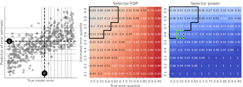
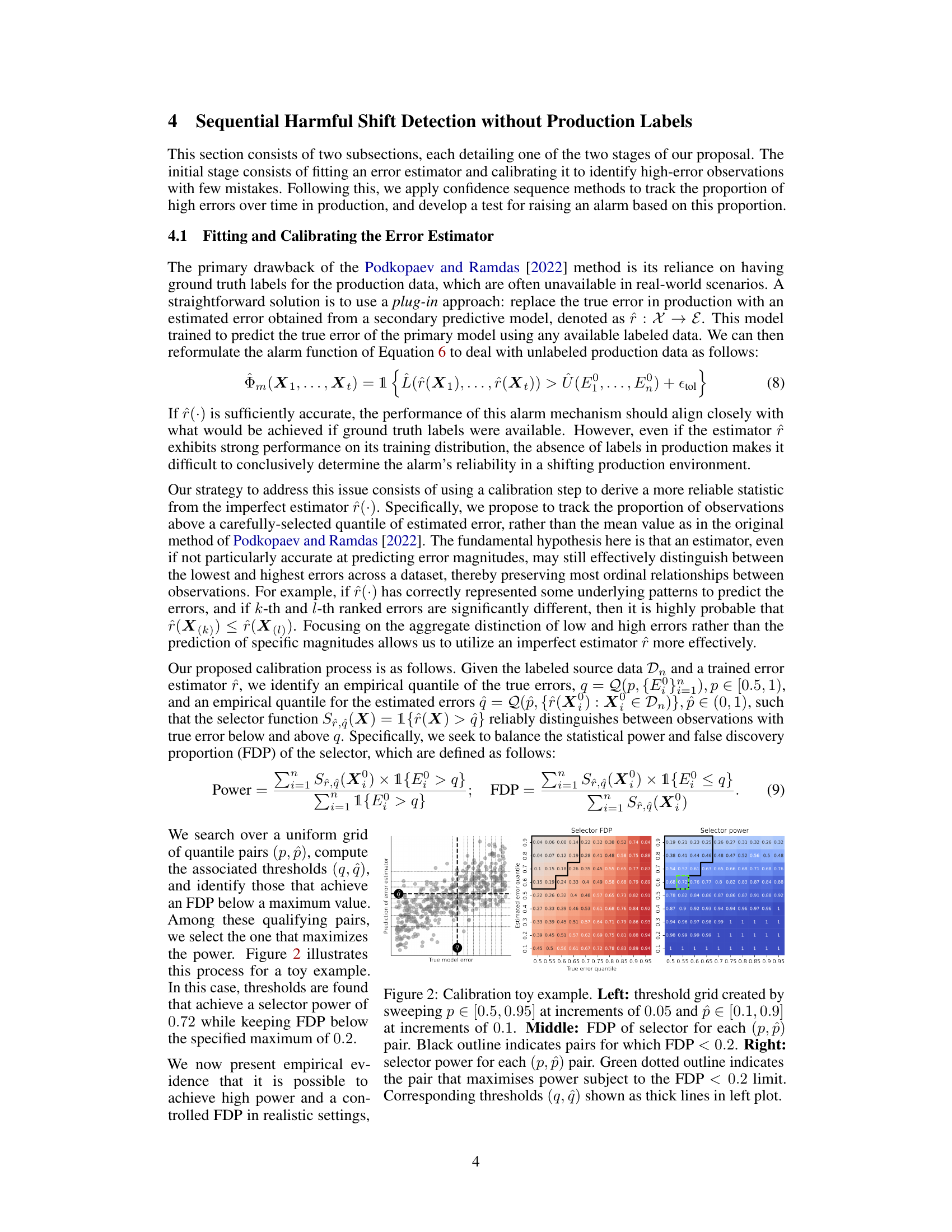
This figure illustrates the calibration process for selecting optimal thresholds to balance statistical power and false discovery proportion (FDP). The left panel shows a grid search over different quantiles of true and estimated errors, represented as (p, p̂). The middle panel displays the FDP for each (p, p̂) pair, highlighting those with FDP below 0.2. The right panel shows the power for each pair, with the optimal pair maximizing power while keeping FDP below 0.2 indicated. The optimal thresholds (q, q̂) are visually highlighted on the left panel.
This figure illustrates the calibration process for selecting optimal thresholds to balance statistical power and false discovery proportion (FDP). The left panel shows a grid search over different quantiles of true and estimated errors. The middle panel displays the FDP for each threshold pair, highlighting pairs with FDP below 0.2. The right panel shows the power for each threshold pair. The optimal threshold pair, maximizing power while keeping FDP below 0.2, is indicated. This process ensures that the selected thresholds effectively distinguish between low and high-error observations, which are then used to track harmful shifts in the production data.
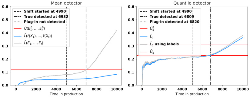
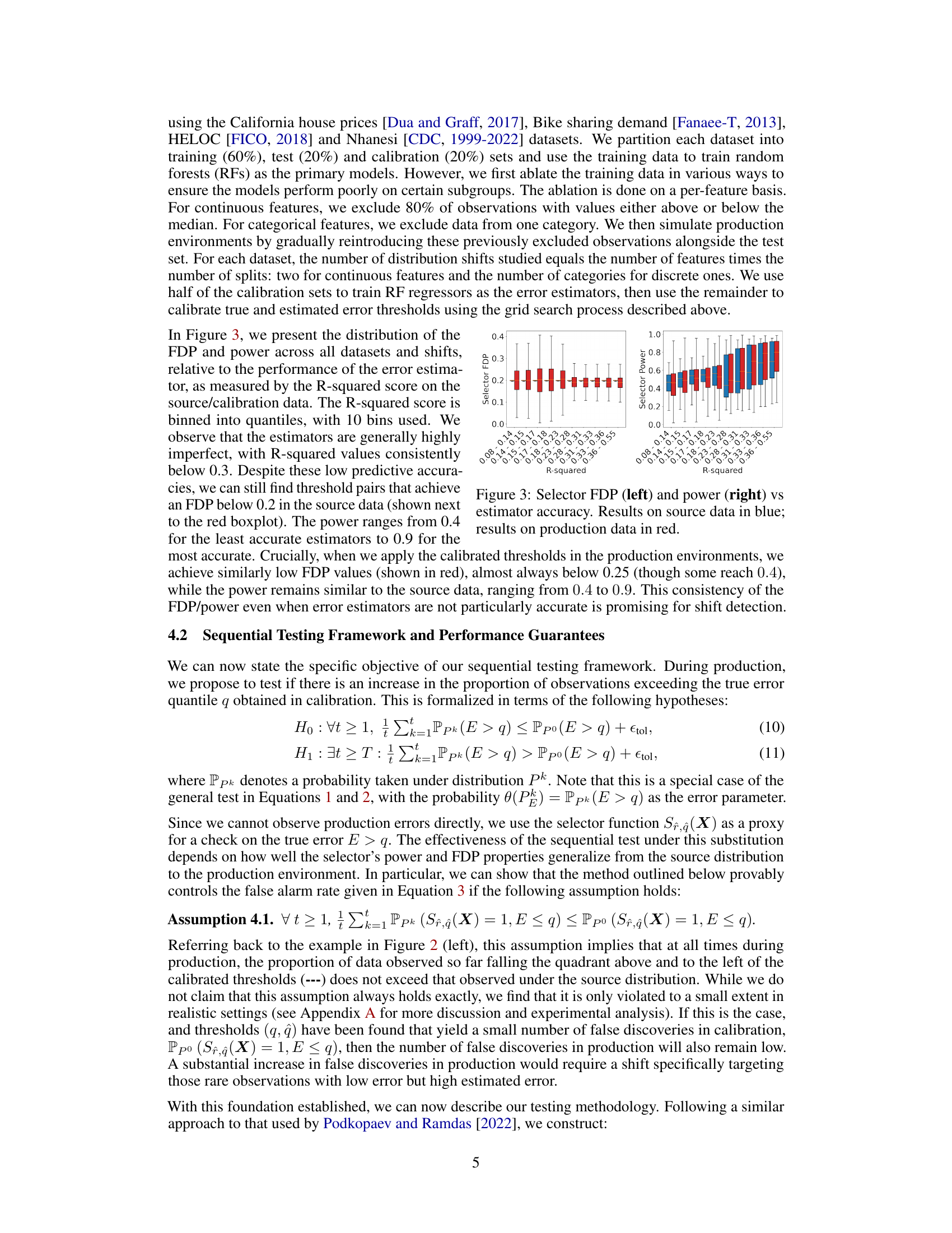
This figure shows the evolution of upper and lower bounds for both the mean and quantile detectors over time in a production setting where a shift occurs. The gray lines represent the lower bounds calculated using the true errors, while the blue lines represent the lower bounds calculated using the estimated errors from the error estimators. The red line indicates the upper bound that must be exceeded for an alarm to be triggered. The pink line in the right panel shows the upper bound of the first statistic for the quantile detector. The figure illustrates the relative performance of the two methods and highlights the difference in detection time due to the reliance on estimated errors in the plug-in approach.

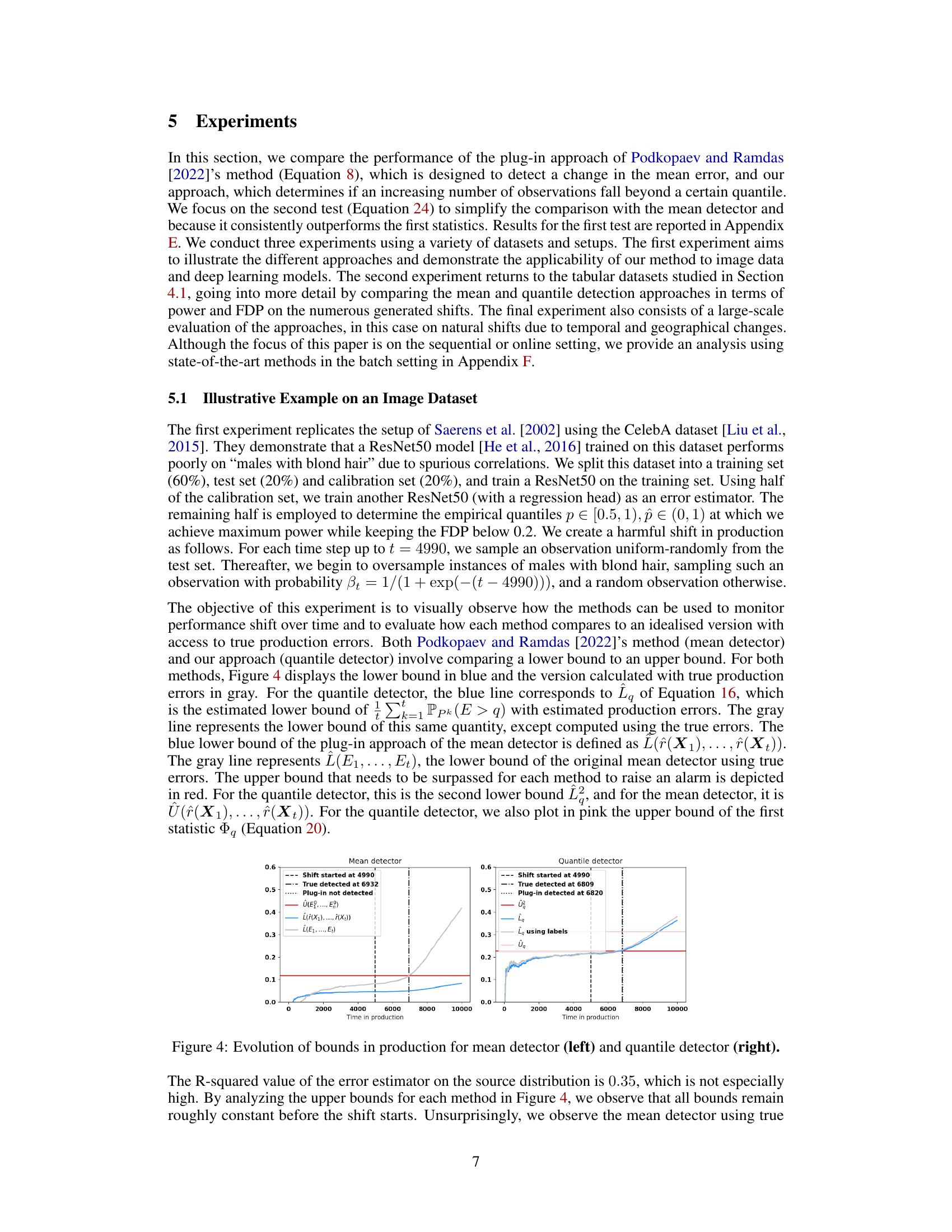
This figure presents a comparison of the quantile and mean detection methods across various datasets and harmfulness thresholds. The left panel shows the power and false discovery proportion (FDP) when the harmfulness threshold is set to zero. The middle panel displays the absolute difference in detection time between the methods using estimated versus true errors. The right panel illustrates the power of each method as the harmfulness threshold varies.

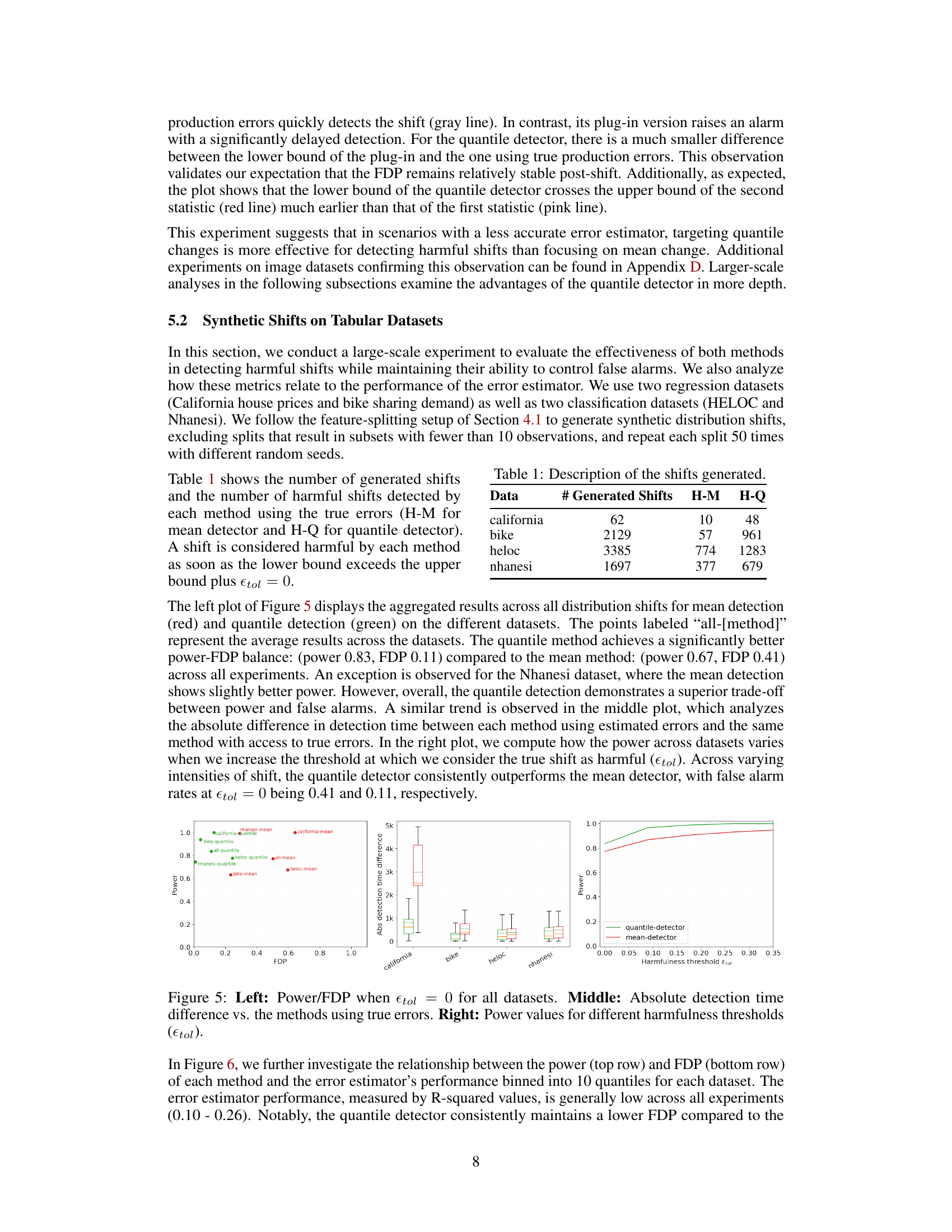
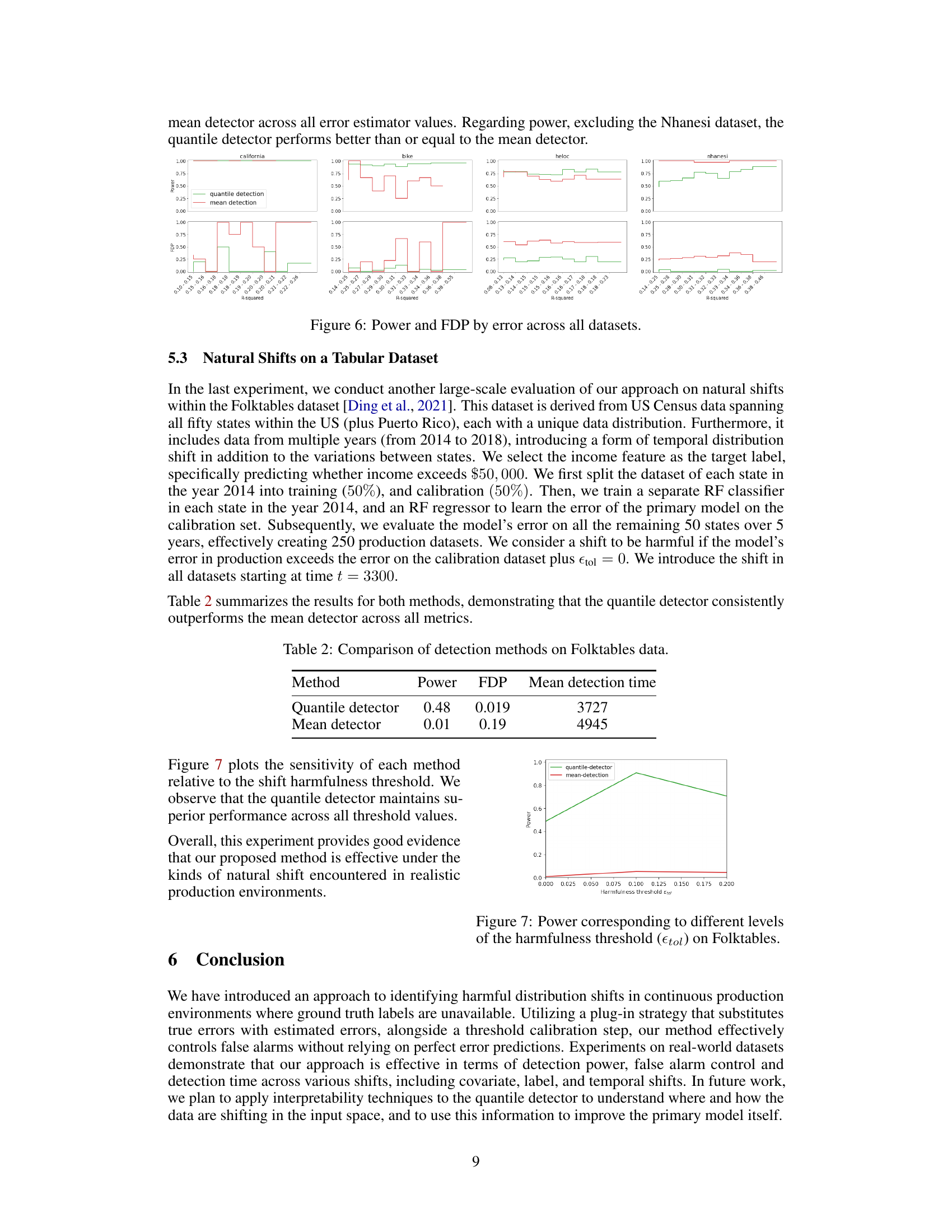
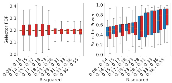
This figure shows the relationship between the power and false discovery proportion (FDP) of both the quantile detector and the mean detector, across different ranges of R-squared values from the error estimator. The R-squared values represent the accuracy of the error estimator, which ranges from 0.1 to 0.55 across all datasets. For each R-squared range, the power and FDP are averaged over all datasets and all the different shift types for both methods. It is used to illustrate how the performance of the error estimator affects both methods. Overall, the figure indicates that the quantile detector maintains lower FDP compared to the mean detector across all datasets and error estimator ranges, while exhibiting comparable or even better power.
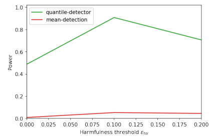
This figure summarizes the results of a large-scale experiment evaluating the effectiveness of both mean and quantile detection methods in detecting harmful shifts while controlling false alarms. It shows the performance of both methods across various datasets and synthetic distribution shifts. The left panel displays the aggregated power and false discovery proportion (FDP) across datasets. The middle panel visualizes the absolute difference in detection time between the methods using estimated versus true errors. The right panel analyzes how the power changes with varying harmfulness threshold, showing the consistent superiority of the quantile detector.

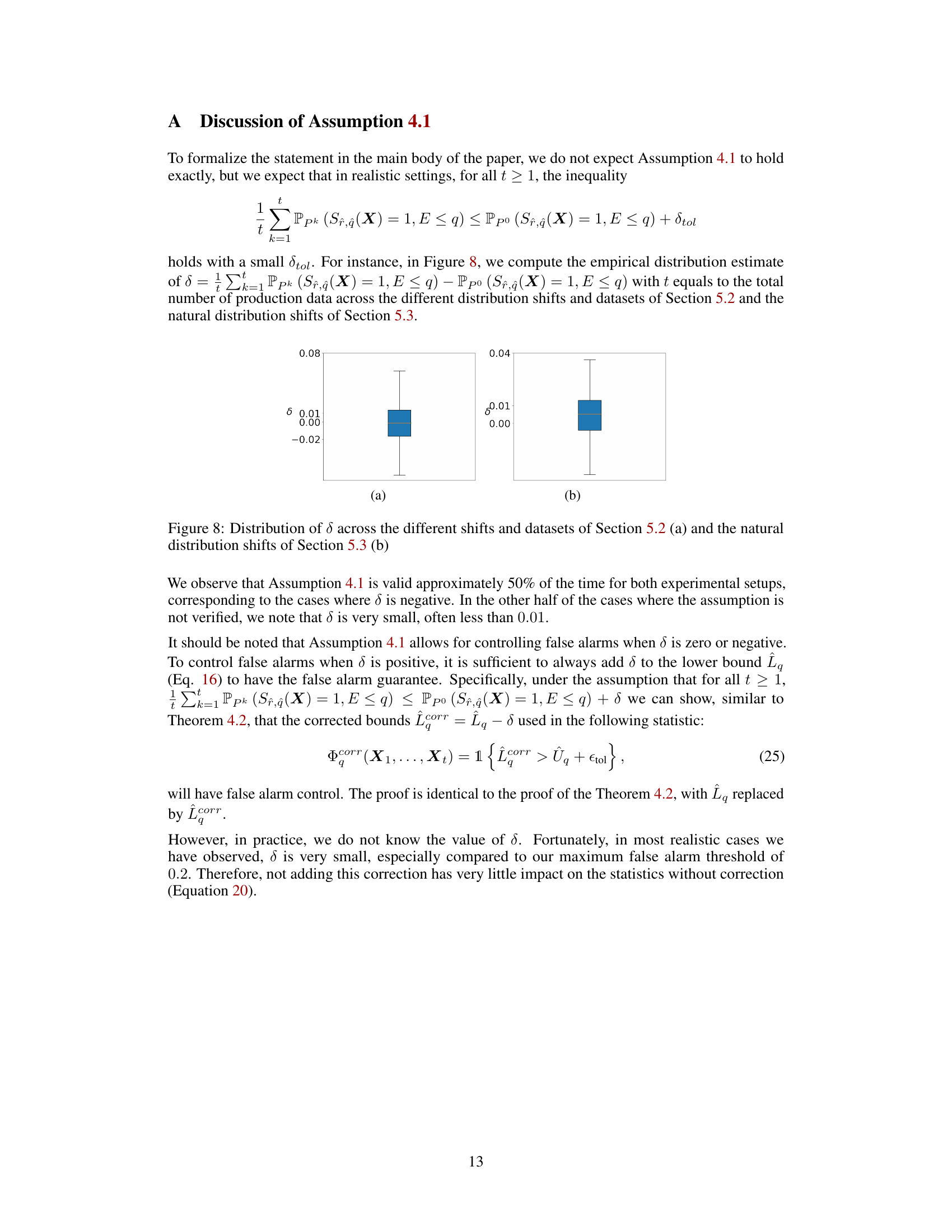
This figure shows the distribution of delta (δ), which represents the difference between the empirical distribution of false positives in production data and that in the source data. Subfigure (a) presents the distribution across synthetic shifts and datasets from Section 5.2, while subfigure (b) displays the distribution across natural shifts from Section 5.3. The box plots illustrate the median, quartiles, and range of δ values, providing insights into the validity of Assumption 4.1 which states that the rate of false positives in production should not exceed that in the source data by much. The figure suggests that Assumption 4.1 holds approximately half the time and when it doesn’t the difference is small.
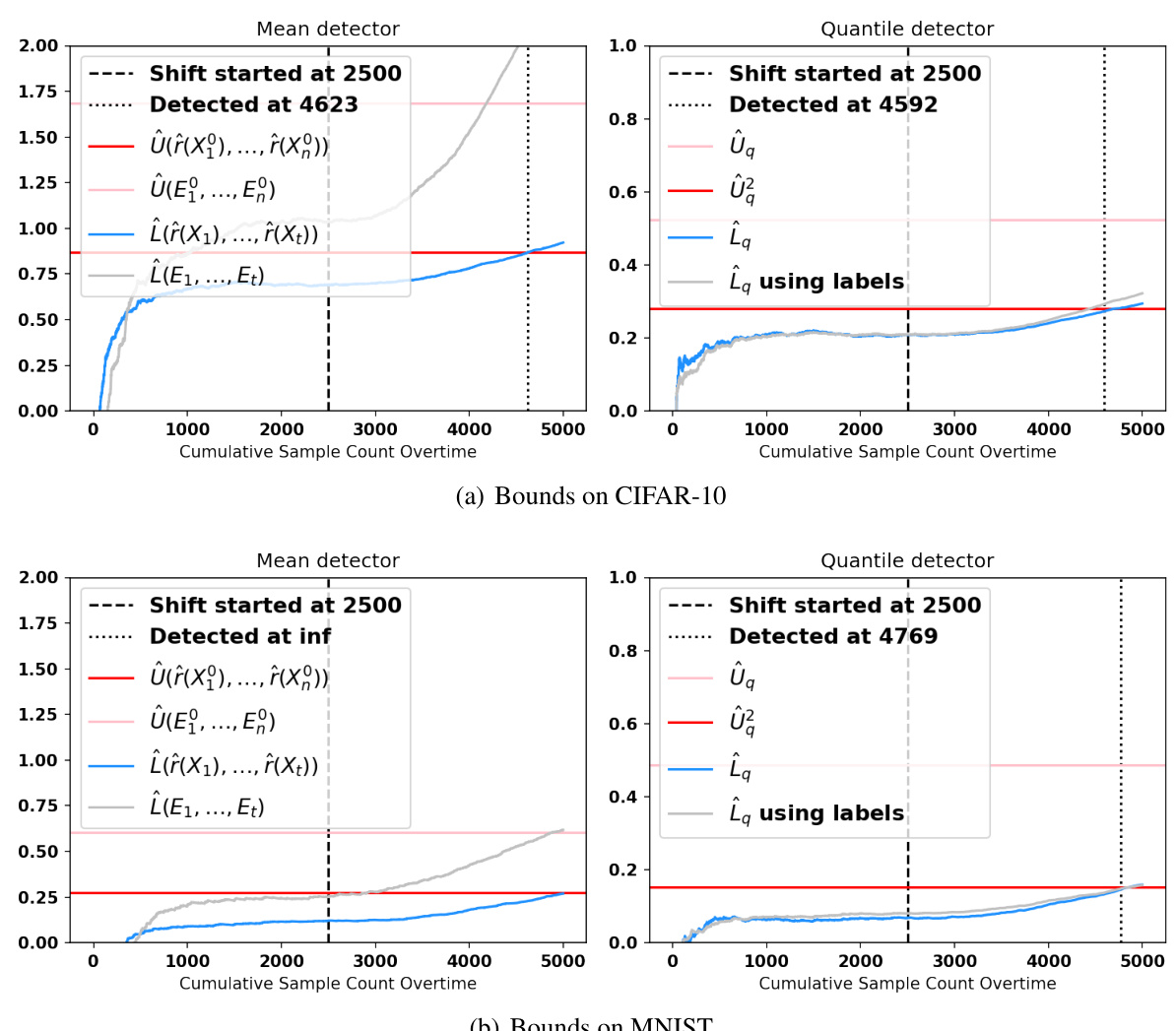
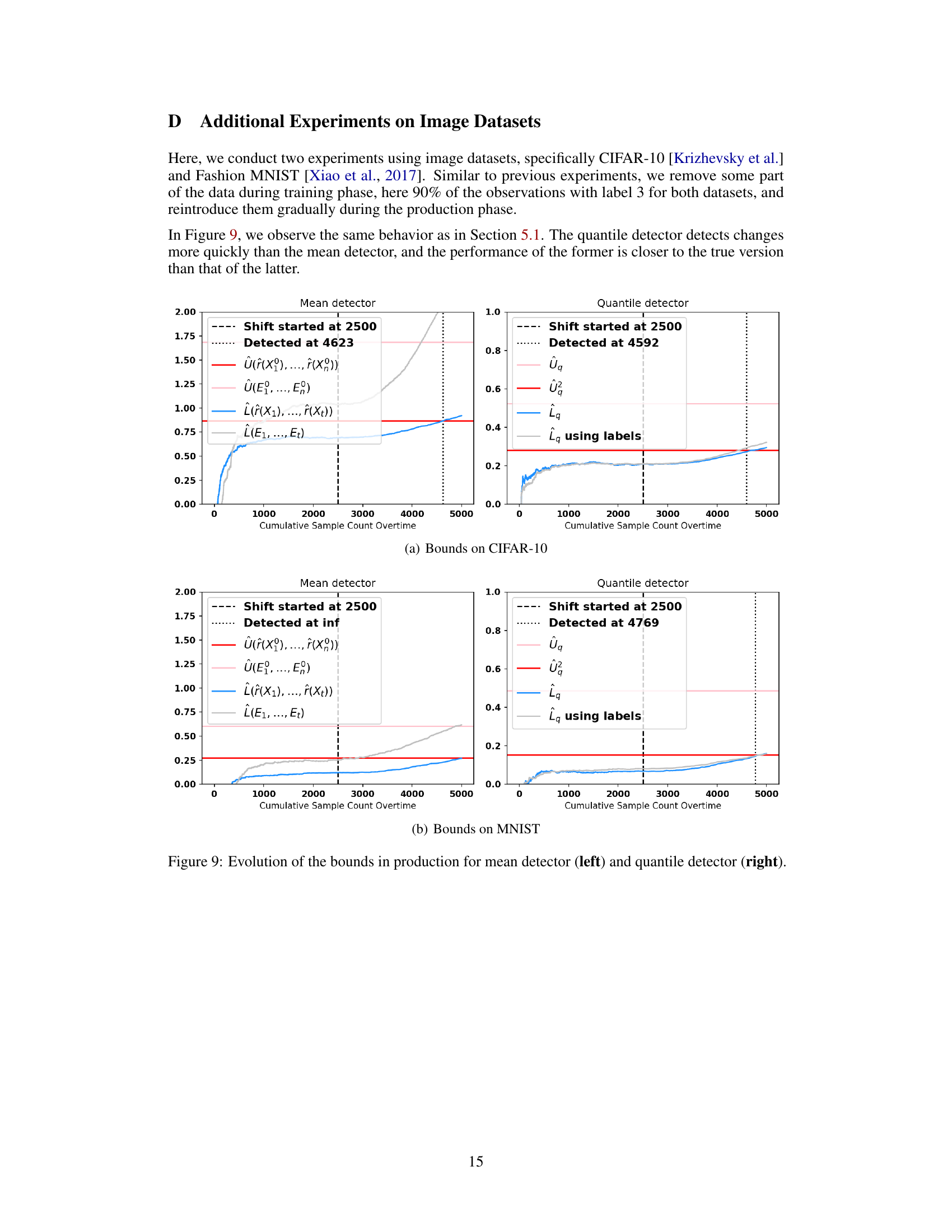
This figure displays the evolution of the upper and lower bounds for both the mean and quantile detectors over time. The upper bound (red line) represents the threshold that must be exceeded to trigger an alarm. The lower bound (blue line) represents the estimated lower bound of the error parameter with access to only estimated errors, and the grey line is based on calculations using the true error. The pink line displays an additional upper bound for the quantile detector, and this line must also be exceeded to raise an alarm for the second test. The figure shows that in both mean and quantile scenarios, the detector using true errors raised alarms earlier than the plug-in version. The quantile detector is closer to the true error detector than the mean detector, especially when the estimator is imperfect.

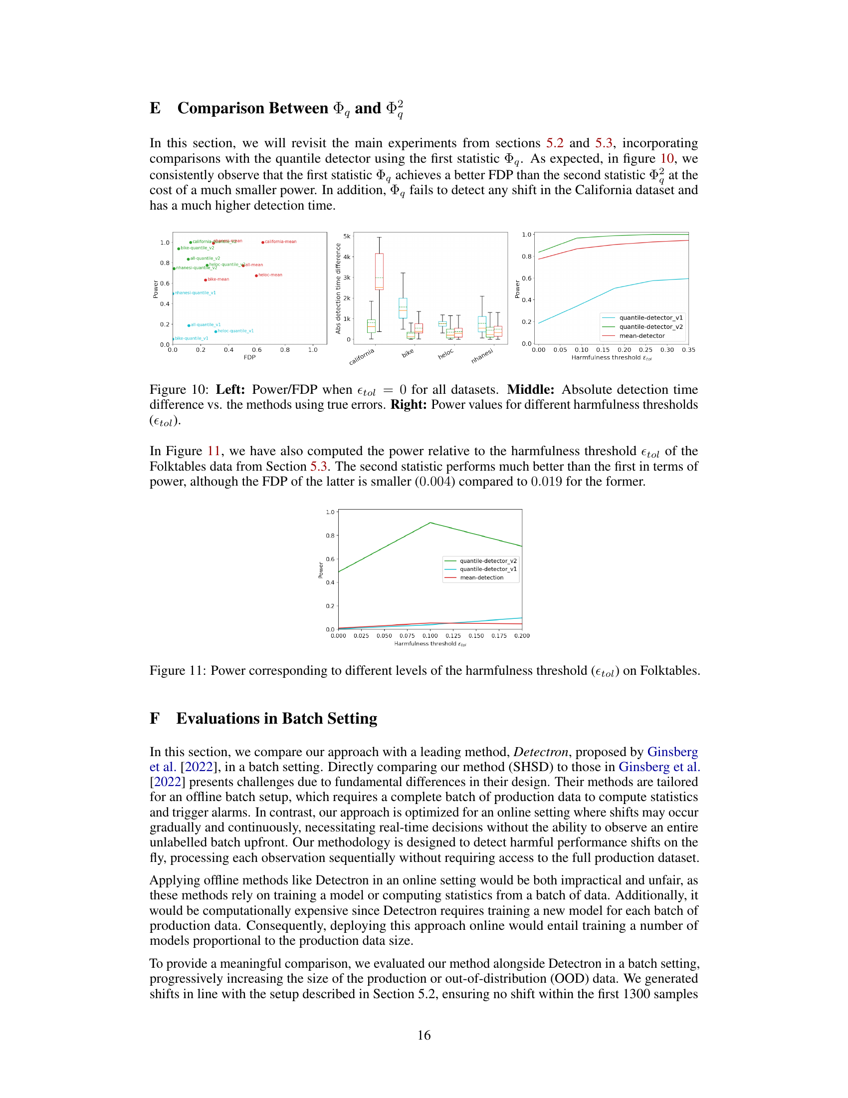
This figure compares the performance of the first and second versions of the quantile detector with the mean detector using three metrics: Power, FDP (False Discovery Proportion), and absolute detection time difference. The left panel shows the power and FDP trade-off for all datasets when the harmfulness threshold is zero. The middle panel displays box plots of the absolute difference in detection time between the methods using estimated errors and the same methods with access to true errors. The right panel illustrates how the power of each method varies across datasets as the harmfulness threshold increases.
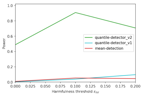
This figure compares the performance of two different quantile detectors (v1 and v2) and a mean detector. The left panel shows the power and false discovery proportion (FDP) when the harmfulness threshold is zero. The middle panel shows the difference in detection time between the methods using estimated and true errors. The right panel shows how power varies across different harmfulness thresholds. The quantile detectors generally exhibit better power-FDP trade-off compared to the mean detector. However, the first quantile detector (v1) performs poorly in terms of power.
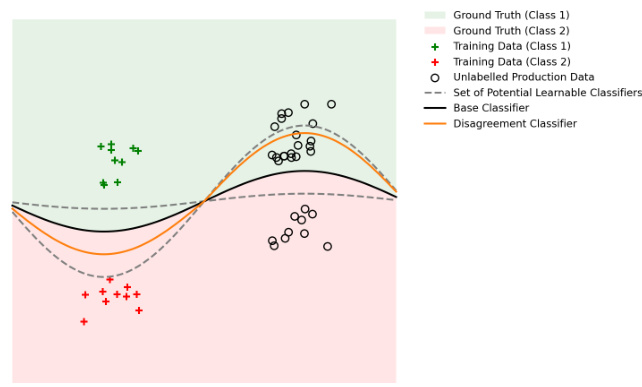
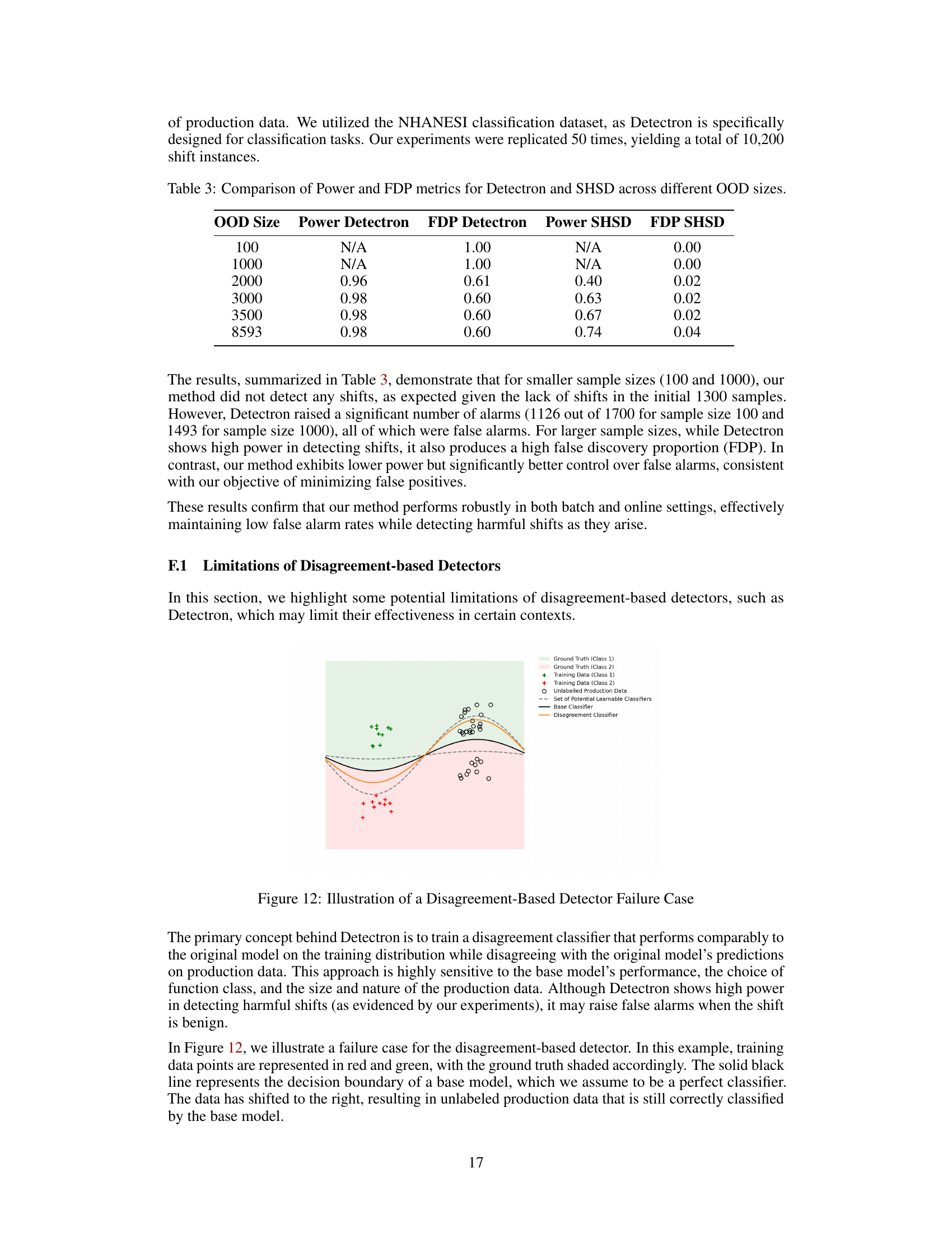
The figure illustrates a scenario where a disagreement-based detector, like Detectron, might fail. Even though the data has shifted (in a benign way), the base classifier (a perfect classifier in this example) still correctly classifies the new data. However, a disagreement classifier might learn to mimic the base classifier’s performance on the training data but disagree on the new data, leading to a false alarm. This highlights the sensitivity of disagreement-based methods to the base model’s performance, the complexity of the disagreement classifier, and the properties of the data.
More on tables

This table presents a comparison of the performance of quantile and mean detection methods on the Folktables dataset. It shows the power (the probability of correctly identifying a harmful shift), the false discovery proportion (FDP, the rate of false positives), and the mean detection time (the average time it takes to detect a harmful shift) for each method. The results demonstrate that the quantile detector outperforms the mean detector in terms of power and FDP while maintaining a reasonable mean detection time.

This table presents a comparison of the performance of Detectron and the proposed SHSD method in detecting harmful distribution shifts, across different sizes of out-of-distribution (OOD) data. The comparison is made using two key metrics: Power (the ability to correctly detect a shift when it occurs) and FDP (False Discovery Proportion, the rate of incorrectly flagging a shift when none is present). The results show that for smaller OOD sizes, Detectron exhibits high FDP while the SHSD method shows no detection ability. However, as the OOD size increases, SHSD method demonstrates superior performance in detecting shifts, maintaining a low FDP while showing increasingly high Power, outperforming Detectron which shows high power at the cost of also having high FDP.
Full paper#
