TL;DR#
Traditional Poisson process models lack flexibility. Gaussian Cox process with GP priors offer more flexibility but suffer from computational complexity and limitations in kernel types and stationarity. Permanental processes improve analytical tractability by using a square link function, but they inherit the cubic complexity and kernel limitations of GPs.
This paper proposes Nonstationary Sparse Spectral Permanental Process (NSSPP) to address the above issues. NSSPP leverages sparse spectral representation of nonstationary kernels to reduce computation to a linear level. A deep kernel variant, DNSSPP, is introduced by stacking multiple spectral mappings, enhancing the model’s ability to capture complex patterns. Empirical results on synthetic and real-world datasets validate the effectiveness of NSSPP and DNSSPP, especially for nonstationary data.
Key Takeaways#
Why does it matter?#
This paper is important because it addresses limitations of existing permanental process models, improving flexibility and efficiency for analyzing point process data. It introduces nonstationary and deep kernel variants, opening avenues for complex data analysis in various applications like neuroscience and finance. The publicly available code further enhances its impact on the research community.
Visual Insights#

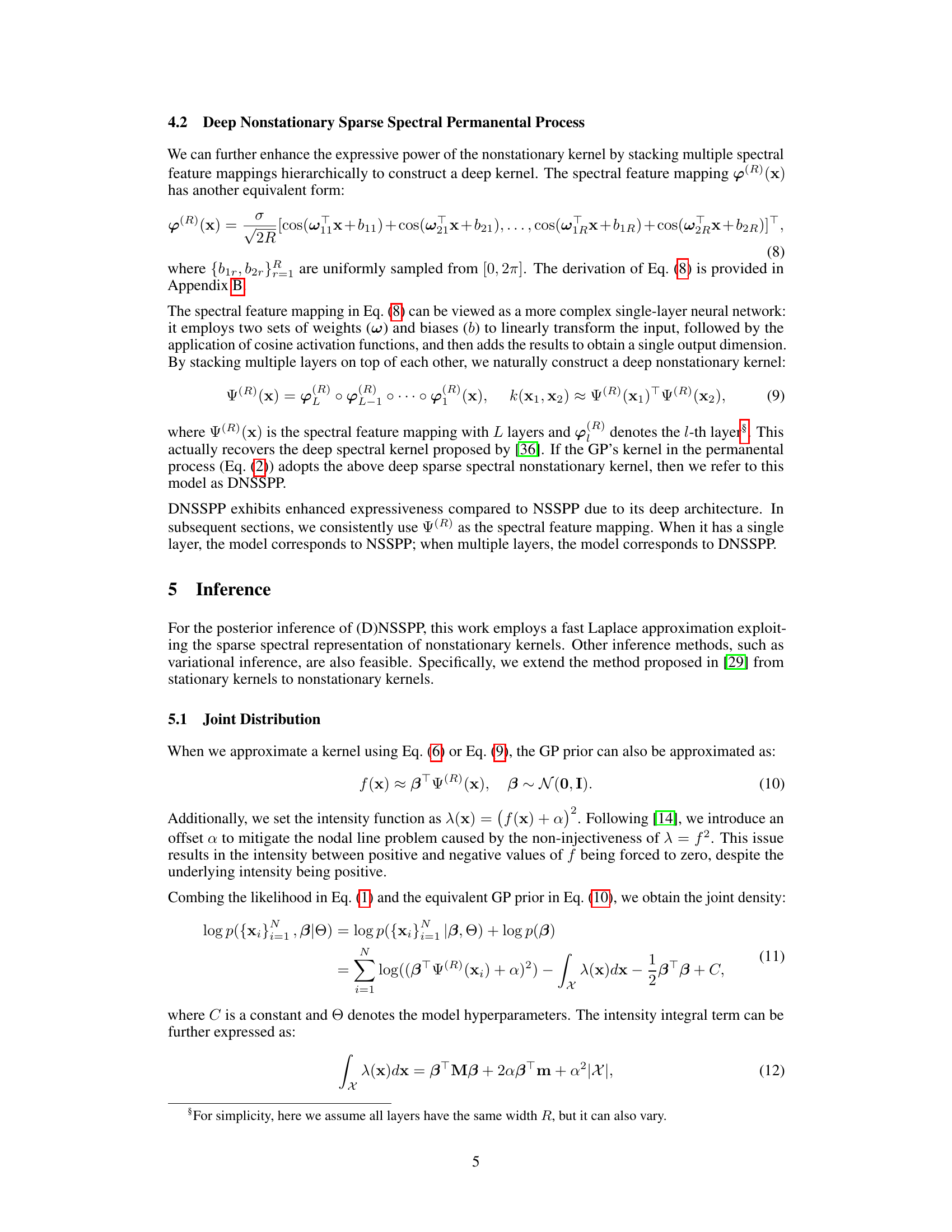
🔼 This figure shows the performance comparison of different models (VBPP, LBPP, SSPP, GSSPP, NSMPP, NSSPP, DNSSPP) on both stationary and nonstationary synthetic datasets. Subfigures (a) and (b) display the fitting results of the intensity functions for each model on stationary and nonstationary data respectively. The plots clearly show the better performance of NSSPP and DNSSPP on nonstationary data. Subfigures (c) and (d) show ablation studies for DNSSPP on nonstationary data, examining the impact of network width/depth and the number of epochs/learning rate on model performance. These subfigures illustrate the effect of hyperparameters on the model’s ability to generalize and avoid overfitting.
read the caption
Figure 1: (a) The fitting results of the intensity functions for all models on the stationary synthetic data; (b) those on the nonstationary synthetic data. The impact of (c) network width and depth, (d) the number of epochs and learning rate on the Ltest of DNSSPP on the nonstationary data.
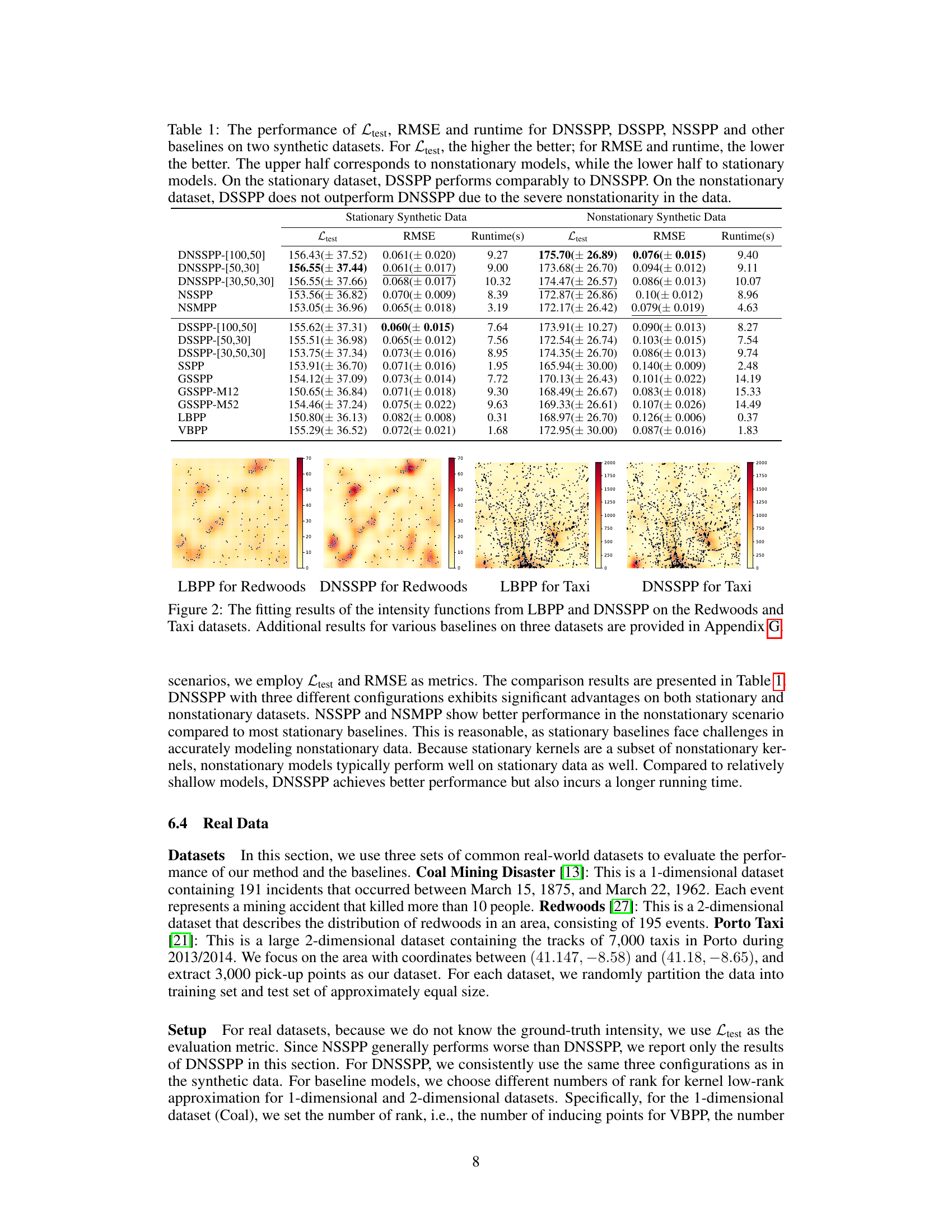
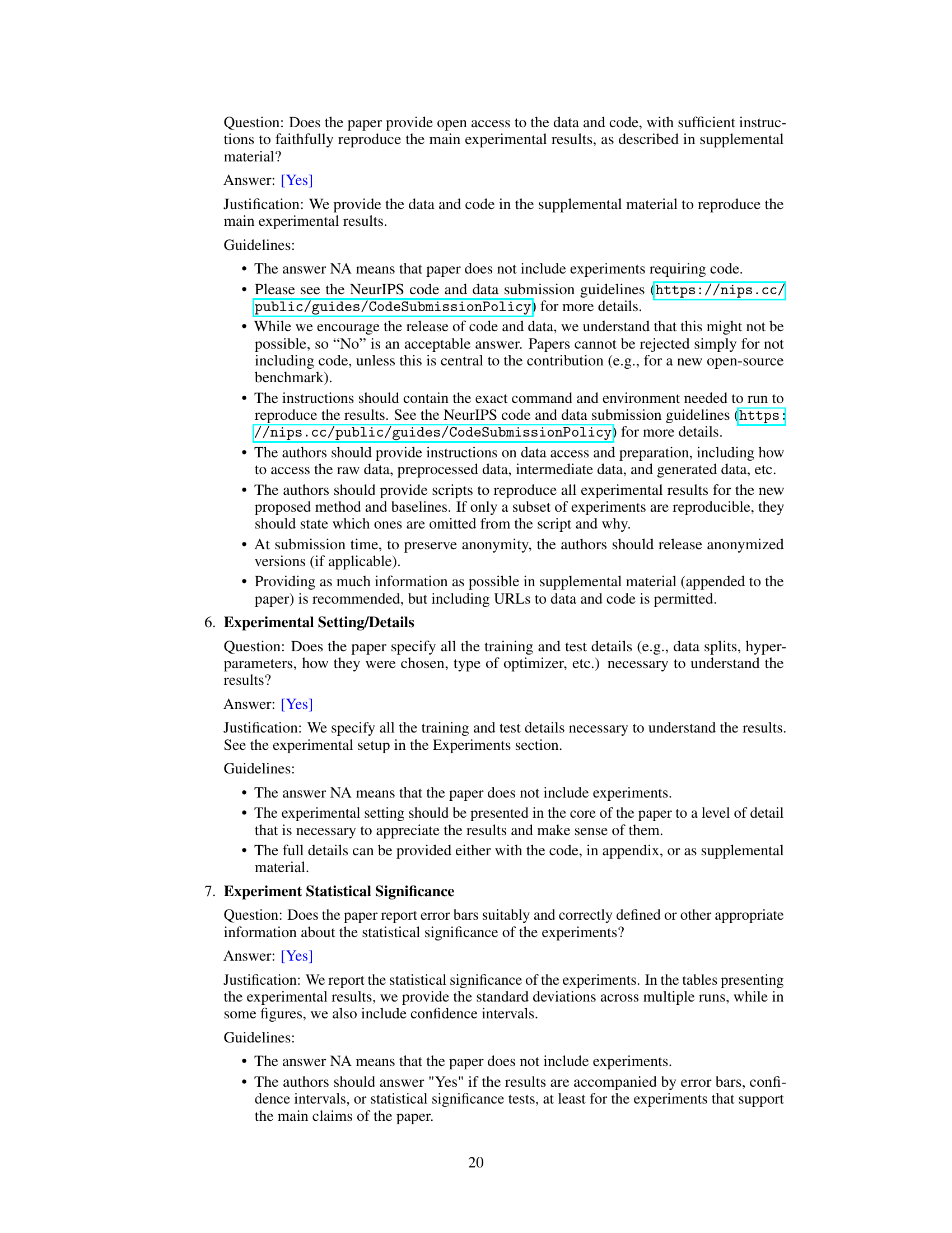
🔼 This table presents the performance comparison of DNSSPP and several baseline models on two synthetic datasets (stationary and nonstationary). The metrics used for comparison are the expected log-likelihood (Ltest), root mean squared error (RMSE), and runtime. Higher Ltest values indicate better performance, while lower RMSE and runtime values are preferred. The results show that DNSSPP generally outperforms other methods, especially on nonstationary data, where its ability to model non-stationarity provides a significant advantage.
read the caption
Table 1: The performance of Ltest, RMSE and runtime for DNSSPP, DSSPP, NSSPP and other baselines on two synthetic datasets. For Ltest, the higher the better; for RMSE and runtime, the lower the better. The upper half corresponds to nonstationary models, while the lower half to stationary models. On the stationary dataset, DSSPP performs comparably to DNSSPP. On the nonstationary dataset, DSSPP does not outperform DNSSPP due to the severe nonstationarity in the data.
In-depth insights#
Sparse Spectral Kernel#
Sparse spectral kernel methods offer a powerful approach to scaling Gaussian processes by approximating the kernel matrix with a low-rank representation. This is achieved by leveraging the spectral representation of the kernel, which decomposes it into a set of eigenfunctions and eigenvalues. The key idea is to select a subset of these eigenfunctions, leading to a sparse representation that significantly reduces computational complexity, while preserving much of the original kernel’s predictive power. This sparsity is crucial for handling large datasets where the full kernel matrix becomes intractable. The effectiveness of sparse spectral methods is heavily dependent on the choice of eigenfunctions and the approximation strategy. Different techniques, like random Fourier features or deterministically selected frequencies, have been proposed and their performance varies depending on the data characteristics and the kernel’s properties. Furthermore, sparse spectral kernels have shown promise in addressing non-stationarity by incorporating spatial variations into the eigenfunctions selection or transformation. This allows for more flexible and expressive models capable of representing complex patterns in non-stationary data. The main challenge lies in balancing the sparsity level to maintain accuracy against the computational cost. Therefore, adapting the appropriate technique and hyperparameters for a specific application remains a critical consideration.
Nonstationary Modeling#
In the realm of temporal data analysis, the assumption of stationarity—that statistical properties remain constant over time—often proves unrealistic. Nonstationary modeling offers crucial advancements by acknowledging and addressing this limitation. It allows for capturing the dynamic evolution of patterns and relationships within data, resulting in more accurate and insightful analyses. Techniques like time-varying parameter models and regime-switching models provide flexible frameworks to handle the changing characteristics of nonstationary processes. These methods effectively capture trends, seasonality, and structural breaks, leading to improved forecasting, anomaly detection, and risk management. Furthermore, incorporating nonstationary features into machine learning algorithms enhances model robustness and predictive performance in diverse fields such as finance, climatology, and epidemiology, where temporal shifts are inherent.
Deep Kernel Variant#
The concept of a “Deep Kernel Variant” in the context of non-stationary sparse spectral permanental processes presents a significant advancement. The core idea involves hierarchically stacking multiple spectral feature mappings to create a deep kernel, thereby dramatically improving the model’s capacity to capture complex patterns in data. This deep architecture enhances expressiveness beyond what’s achievable with traditional shallow kernels, overcoming limitations in representing intricate relationships. While the resulting intensity integral loses its analytical solvability, necessitating numerical integration, the gain in representational power likely outweighs this computational cost, especially for datasets exhibiting strong non-stationarity. The trade-off between computational complexity and model expressiveness is a key consideration here, with the deep kernel variant offering a pathway to superior performance in more challenging scenarios. The effectiveness of this approach hinges on careful hyperparameter tuning (e.g., network depth, width) to avoid overfitting. Further research could investigate optimal network architectures and training strategies for this deep kernel to maximize its potential.
Laplace Approximation#
The Laplace approximation, employed to estimate the posterior distribution of model parameters, is a crucial aspect of the presented work. Its use streamlines the inference process by approximating the complex, high-dimensional posterior with a simpler Gaussian distribution. This approximation hinges on a second-order Taylor expansion around the posterior’s mode (maximum), significantly reducing computational demands, particularly beneficial when dealing with large datasets. While the Laplace method offers computational efficiency, it also introduces approximation errors, potentially impacting accuracy. The paper acknowledges this limitation, and the trade-off between computational feasibility and precision is implicit in their approach. The choice to utilize the Laplace approximation is justified by its suitability for handling the challenges inherent in Bayesian inference for point processes. The authors effectively leverage this technique to provide a scalable and tractable method for posterior estimation in their proposed non-stationary sparse spectral permanental process.
Ablation Study#
An ablation study systematically removes components of a model to assess their individual contributions. In the context of this research paper on Nonstationary Sparse Spectral Permanental Processes, such a study would likely involve removing or altering key aspects of the model’s architecture and comparing performance against a fully functional model. This would help determine the effect of different elements, such as the nonstationary kernel, the sparse spectral representation, and the depth of the network. Removing the nonstationary kernel and reverting to a stationary one would quantify the model’s improvement when dealing with nonstationary data. By testing shallow versus deep kernel variants, the researchers could validate the effectiveness of the deep kernel architecture in capturing complex patterns. Additionally, altering hyperparameters like the number of frequencies in the spectral representation or the depth of the network architecture would be examined to determine the model’s sensitivity to these parameters and to find the optimal configurations. The results would provide valuable insights into which components are essential for the model’s success and which aspects could potentially be simplified or removed without significant performance degradation. Ultimately, the ablation study serves to improve the model’s design, improve its efficiency and to provide a better understanding of how the different aspects interact.
More visual insights#
More on figures
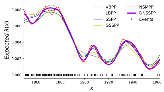
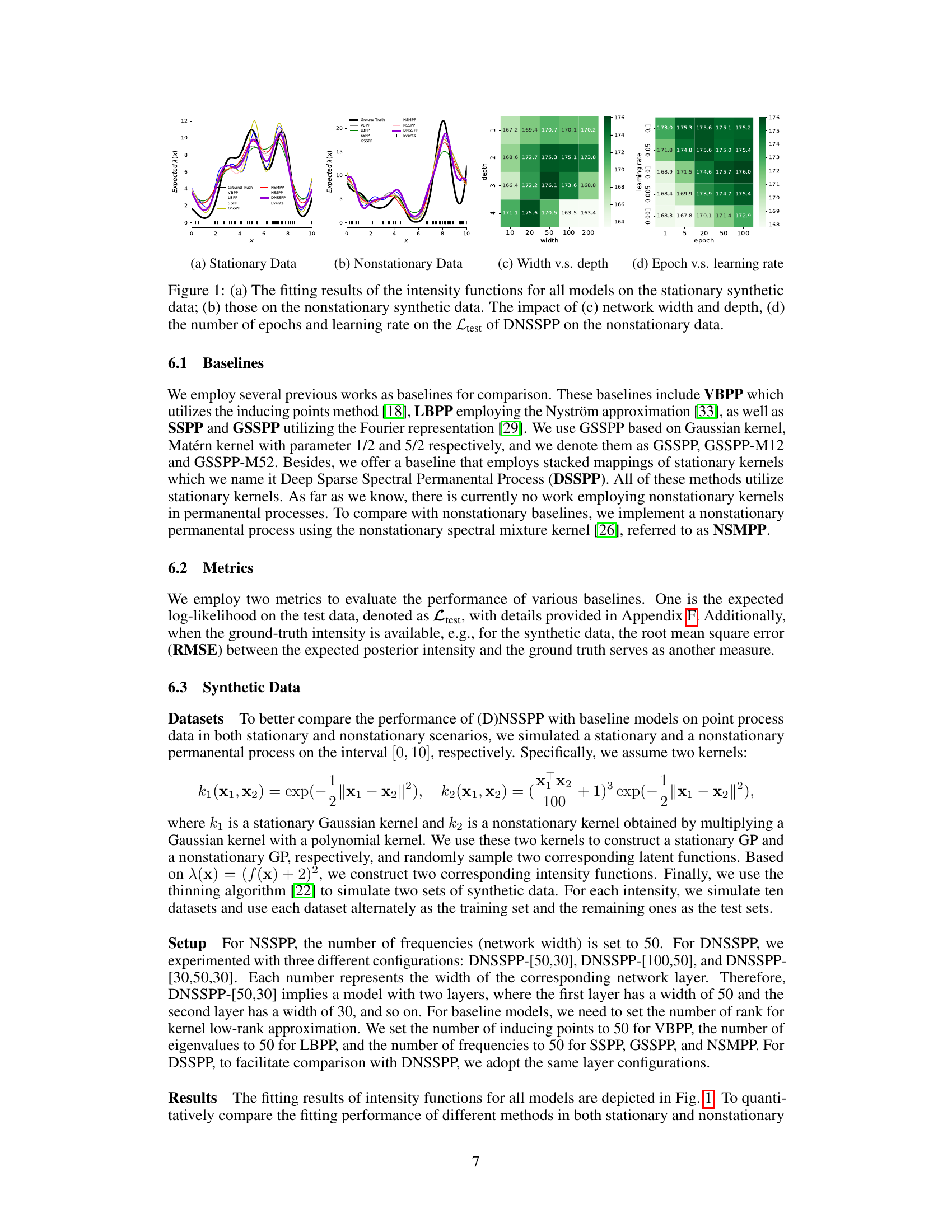
🔼 This figure shows the performance comparison of various models (VBPP, LBPP, SSPP, GSSPP, NSMPP, NSSPP, DNSSPP) on both stationary and nonstationary synthetic datasets. Subfigures (a) and (b) display the fitted intensity functions against the ground truth for each model on stationary and nonstationary data respectively. The model’s ability to accurately capture the intensity function is apparent. Subfigures (c) and (d) show ablation studies on the DNSSPP model exploring how hyperparameters such as network width/depth, number of epochs, and learning rate affect the model’s performance (Ltest metric) on the nonstationary data.
read the caption
Figure 1: (a) The fitting results of the intensity functions for all models on the stationary synthetic data; (b) those on the nonstationary synthetic data. The impact of (c) network width and depth, (d) the number of epochs and learning rate on the Ltest of DNSSPP on the nonstationary data.

🔼 This figure presents the results of applying various models, including the proposed DNSSPP and several baselines, to both stationary and nonstationary synthetic datasets. Subfigures (a) and (b) compare the intensity function estimates of different models against the ground truth for stationary and nonstationary data respectively. Subfigures (c) and (d) illustrate ablation studies showing the impact of network architecture (width and depth) and training hyperparameters (epochs and learning rate) on the performance of the DNSSPP model, specifically on the nonstationary data.
read the caption
Figure 1: (a) The fitting results of the intensity functions for all models on the stationary synthetic data; (b) those on the nonstationary synthetic data. The impact of (c) network width and depth, (d) the number of epochs and learning rate on the Ltest of DNSSPP on the nonstationary data.

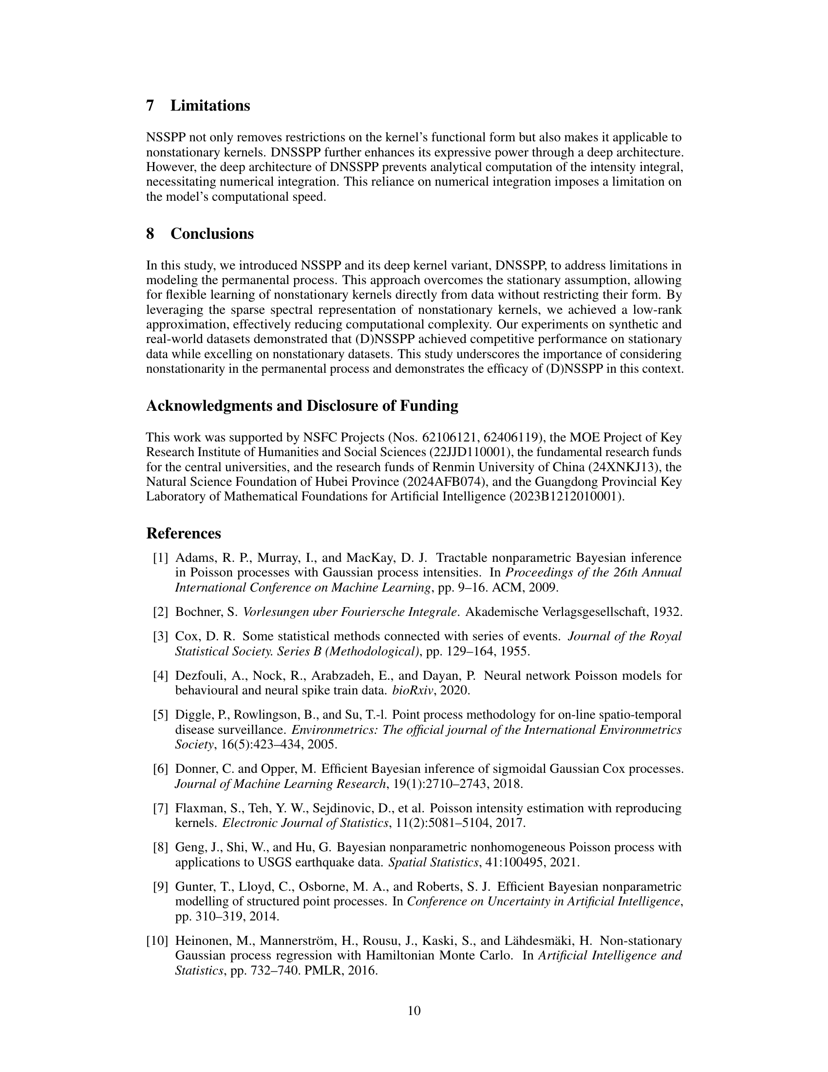
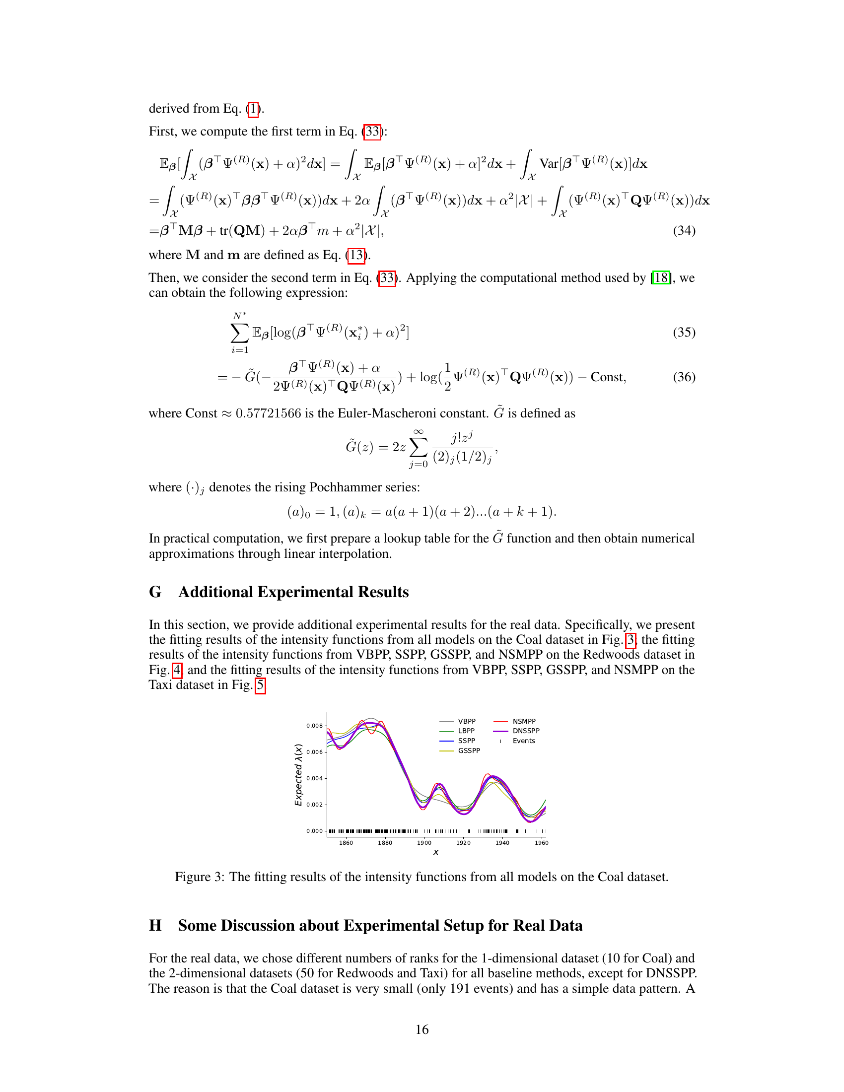
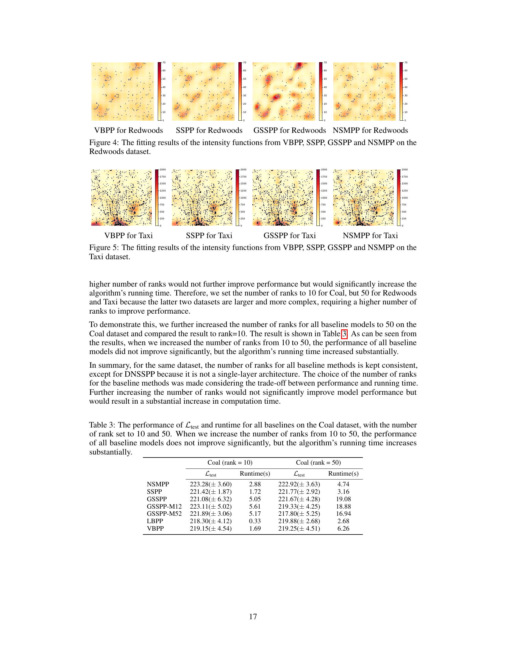
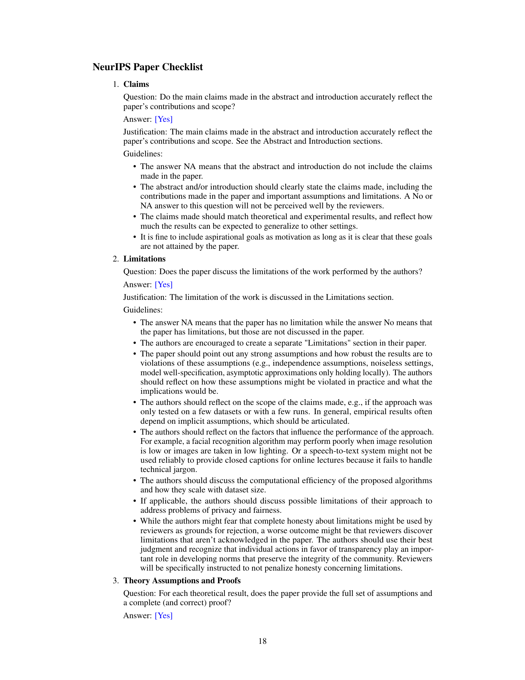
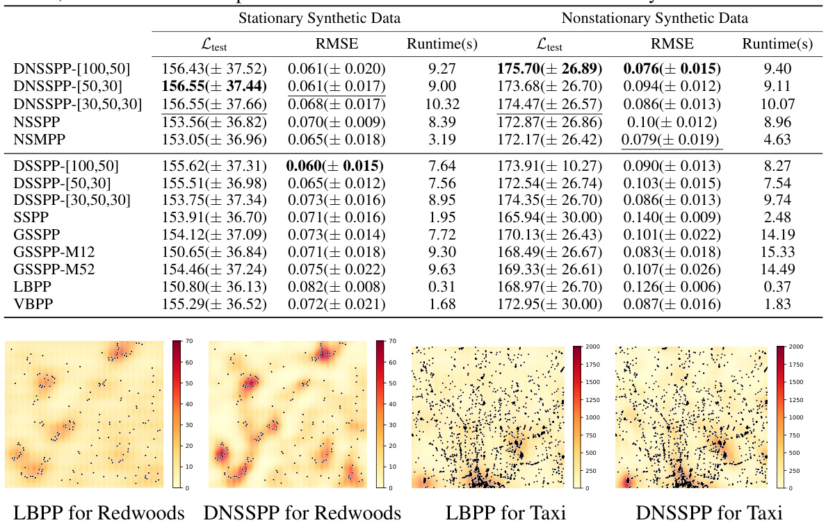
🔼 This figure compares the performance of LBPP and DNSSPP on two real-world datasets: Redwoods and Taxi. It visualizes how well each model’s estimated intensity function matches the actual distribution of events. The Appendix G contains additional results for other baseline methods on these and other datasets, offering a more comprehensive comparison.
read the caption
Figure 2: The fitting results of the intensity functions from LBPP and DNSSPP on the Redwoods and Taxi datasets. Additional results for various baselines on three datasets are provided in Appendix G.
More on tables

🔼 This table presents a comparison of the performance of DNSSPP (Deep Nonstationary Sparse Spectral Permanental Process), DSSPP, NSSPP, and other baseline models on two synthetic datasets: one stationary and one nonstationary. The evaluation metrics include Ltest (expected log-likelihood), RMSE (root mean squared error), and runtime. Higher Ltest values are better, while lower RMSE and runtime values are preferred. The results show that DNSSPP generally outperforms other methods, particularly on the nonstationary dataset, highlighting its ability to handle non-stationary data effectively.
read the caption
Table 1: The performance of Ltest, RMSE and runtime for DNSSPP, DSSPP, NSSPP and other baselines on two synthetic datasets. For Ltest, the higher the better; for RMSE and runtime, the lower the better. The upper half corresponds to nonstationary models, while the lower half to stationary models. On the stationary dataset, DSSPP performs comparably to DNSSPP. On the nonstationary dataset, DSSPP does not outperform DNSSPP due to the severe nonstationarity in the data.

🔼 This table presents the performance comparison of DNSSPP against other baseline models (including DSSPP, NSSPP, and several others) on two synthetic datasets: one stationary and one non-stationary. The comparison is based on three metrics: Ltest (expected log-likelihood, higher is better), RMSE (root mean squared error, lower is better), and runtime (seconds, lower is better). The table’s structure is divided into two halves: the upper half shows the results for non-stationary models, while the lower half shows the results for stationary models. The results highlight DNSSPP’s superior performance, particularly on the non-stationary dataset.
read the caption
Table 1: The performance of Ltest, RMSE and runtime for DNSSPP, DSSPP, NSSPP and other baselines on two synthetic datasets. For Ltest, the higher the better; for RMSE and runtime, the lower the better. The upper half corresponds to nonstationary models, while the lower half to stationary models. On the stationary dataset, DSSPP performs comparably to DNSSPP. On the nonstationary dataset, DSSPP does not outperform DNSSPP due to the severe nonstationarity in the data.
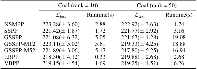
🔼 This table presents the performance comparison of DNSSPP against several baselines on synthetic datasets, both stationary and non-stationary. It shows the Ltest (log-likelihood), RMSE (root mean squared error), and runtime for each model. The results highlight DNSSPP’s superior performance on non-stationary data compared to stationary baselines, while maintaining comparable performance on stationary data.
read the caption
Table 1: The performance of Ltest, RMSE and runtime for DNSSPP, DSSPP, NSSPP and other baselines on two synthetic datasets. For Ltest, the higher the better; for RMSE and runtime, the lower the better. The upper half corresponds to nonstationary models, while the lower half to stationary models. On the stationary dataset, DSSPP performs comparably to DNSSPP. On the nonstationary dataset, DSSPP does not outperform DNSSPP due to the severe nonstationarity in the data.
Full paper#
