TL;DR#
Many applications benefit from diffusion models’ ability to represent complex data distributions. However, their training typically demands extensive clean datasets, which are often unavailable in practical settings. This limitation restricts the use of diffusion models for real-world inverse problems, like image reconstruction from noisy or incomplete observations.
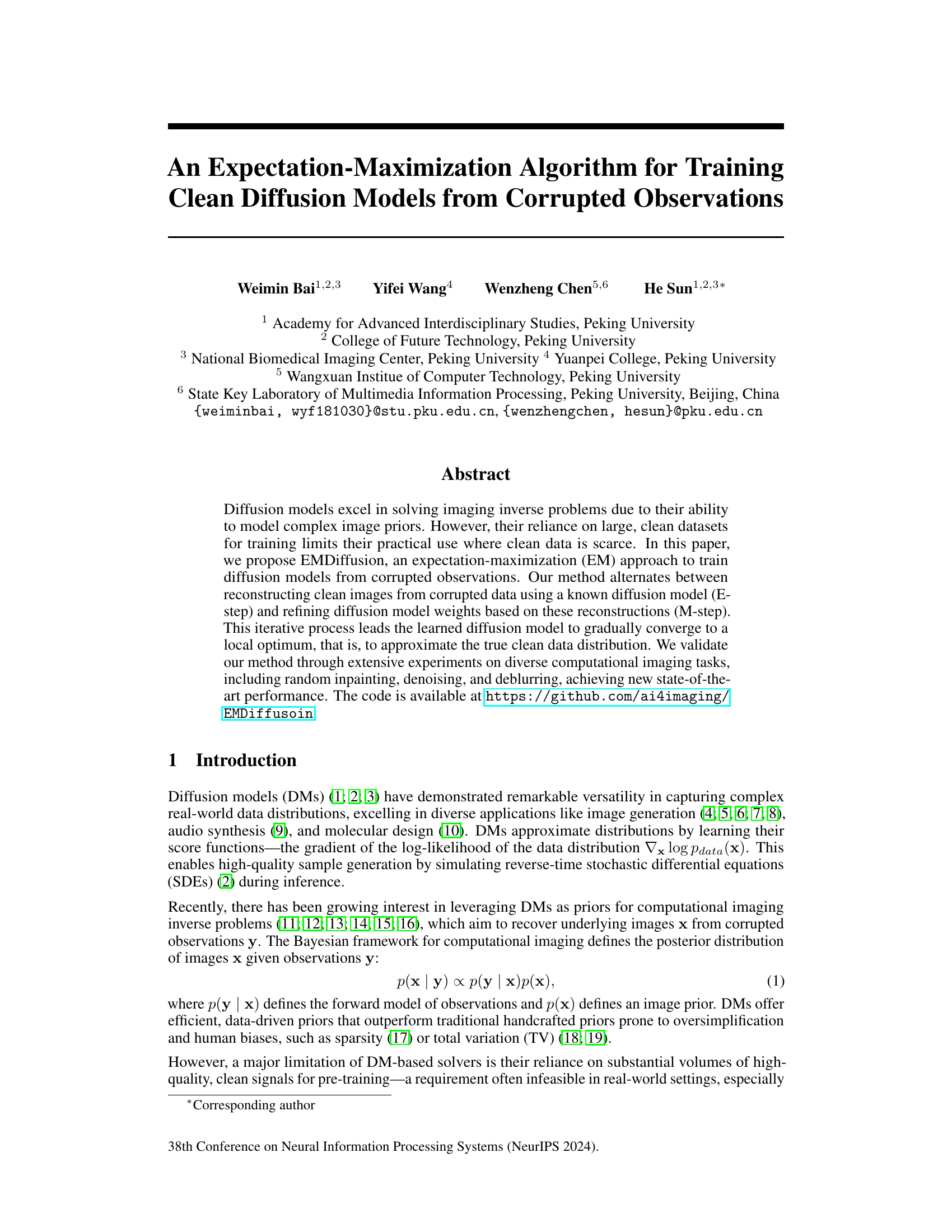
The proposed solution is EMDiffusion, which tackles this issue by using an expectation-maximization (EM) algorithm. This iterative algorithm alternates between reconstructing clean images from corrupted data (E-step) and refining the diffusion model parameters based on these reconstructions (M-step). The incorporation of adaptive diffusion posterior sampling further enhances the algorithm’s performance. The results demonstrate that EMDiffusion achieves state-of-the-art performance on diverse imaging tasks, showing its effectiveness in training high-quality diffusion models from readily available corrupted data.
Key Takeaways#
Why does it matter?#
This paper is crucial for researchers working on diffusion models and inverse problems because it presents a novel solution for training these models using only corrupted data. This significantly expands the applicability of diffusion models to real-world scenarios where obtaining large, clean datasets is often impractical or impossible. The EM approach and adaptive posterior sampling techniques are highly valuable contributions to the field and will likely influence future work.
Visual Insights#
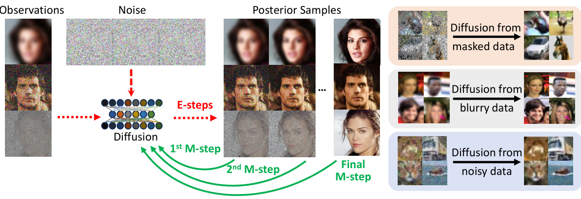
🔼 This figure illustrates the EMDiffusion process. The left side shows the Expectation-Maximization (EM) algorithm iteratively reconstructing clean images from corrupted observations (E-step) and refining the diffusion model weights (M-step). The right side displays examples of raw observations and the corresponding clean images reconstructed by the learned diffusion model.
read the caption
Figure 1: Overview of EMDiffusion. The paper proposes an expectation-maximization (EM) approach to jointly solve imaging inverse problems and train a diffusion model from corrupted observations. Left: In each E-step, we assume a known diffusion model and perform posterior sampling to reconstruct images from corrupted observations. In the M-step, we update the weights of the diffusion model based on these posterior samples. By iteratively alternating between these two steps, the diffusion model gradually learns the clean image distribution and generates high-quality posterior samples. Right: Raw observations and reconstructed clean images based on the diffusion model learned from corrupted data.

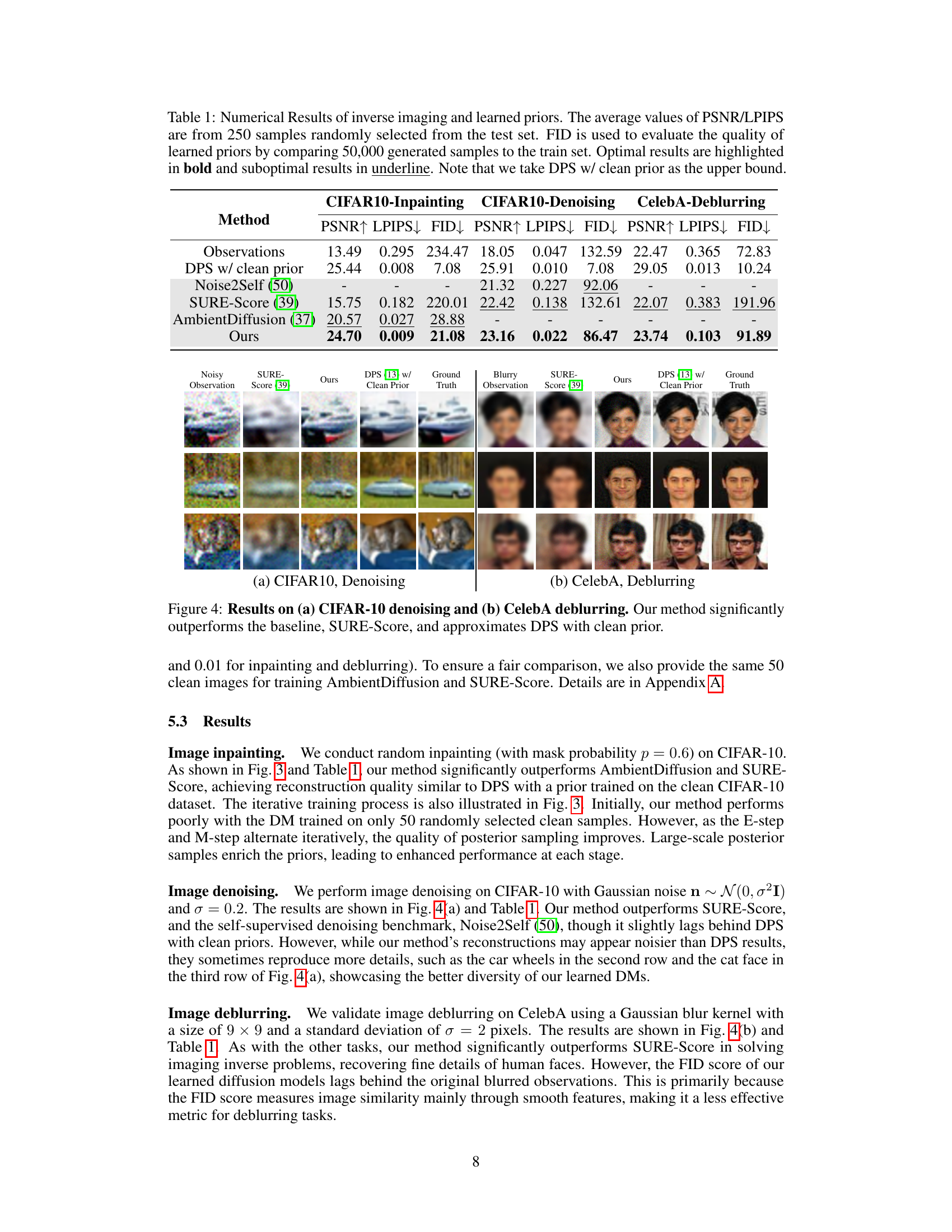
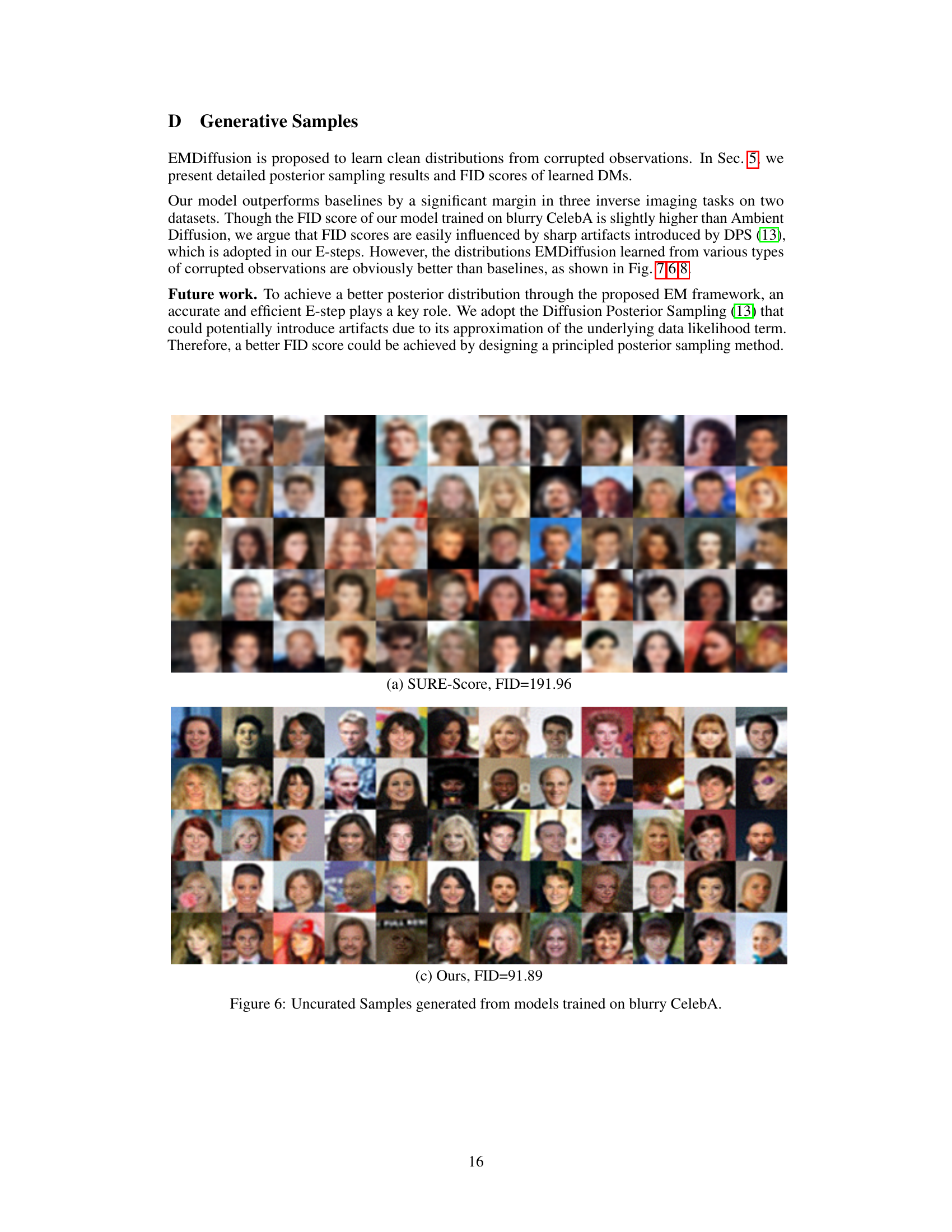
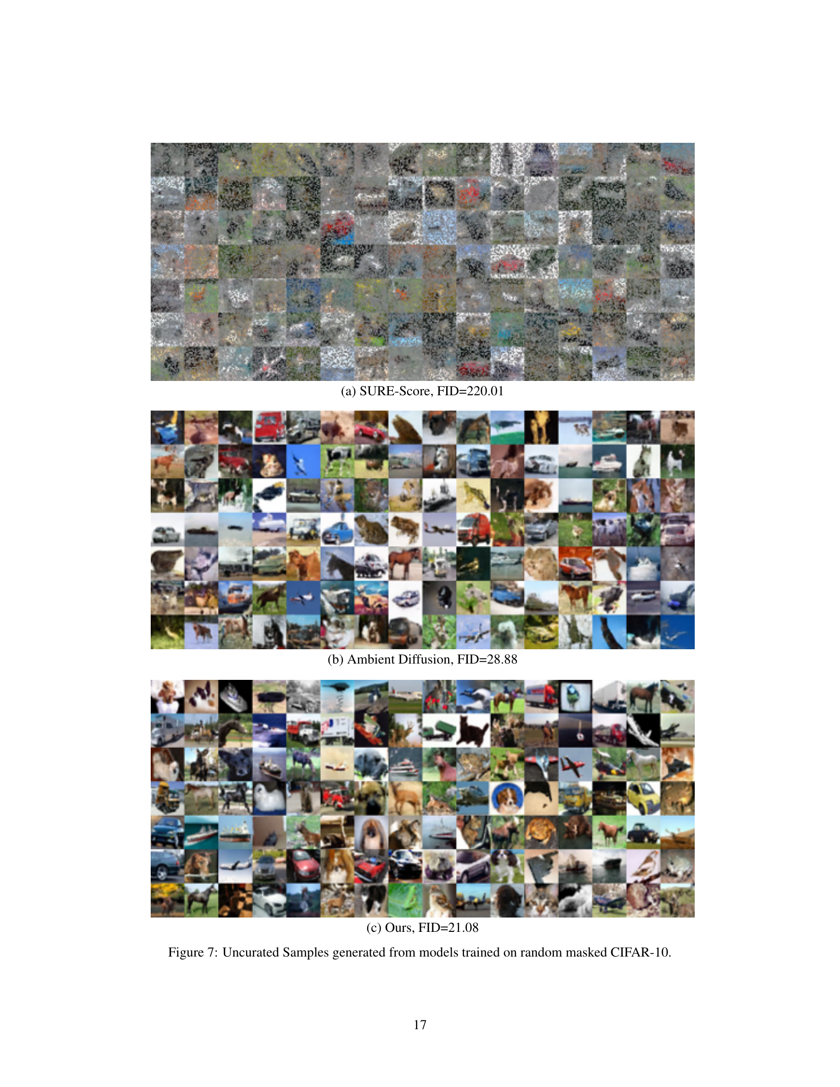
🔼 This table presents a quantitative comparison of different methods for inverse imaging tasks, including inpainting, denoising and deblurring, using CIFAR-10 and CelebA datasets. The metrics used are PSNR (Peak Signal-to-Noise Ratio), LPIPS (Learned Perceptual Image Patch Similarity), and FID (Fréchet Inception Distance), which measure reconstruction quality, perceptual similarity and the quality of generated samples by learned diffusion models respectively. The table shows that the proposed method (Ours) achieves state-of-the-art performance across all tasks, outperforming baselines like SURE-Score and AmbientDiffusion while approximating the results of DPS with clean data.
read the caption
Table 1: Numerical Results of inverse imaging and learned priors. The average values of PSNR/LPIPS are from 250 samples randomly selected from the test set. FID is used to evaluate the quality of learned priors by comparing 50,000 generated samples to the train set. Optimal results are highlighted in bold and suboptimal results in underline. Note that we take DPS w/ clean prior as the upper bound.
In-depth insights#
EM Algorithm for DMs#
The application of the Expectation-Maximization (EM) algorithm to Diffusion Models (DMs) presents a powerful approach to training these models using corrupted data. The core idea is iterative: the E-step reconstructs clean data from noisy observations using a current DM, while the M-step refines the DM parameters based on these reconstructions. This elegantly sidesteps the common limitation of DMs requiring large, clean datasets for training. By iteratively refining the DM’s understanding of the clean data distribution through this EM process, the model can effectively learn from noisy or incomplete observations, expanding the applicability of DMs to real-world scenarios where perfect data is scarce. The EM framework addresses a key challenge: the ‘chicken-and-egg’ problem of needing a good DM to clean the data for effective DM training. The efficacy of this approach rests on the quality of the initial DM, often trained on a smaller subset of clean data; thus, initialization techniques become crucial for achieving optimal performance. Further research should focus on improving initialization strategies and exploring variations of the EM approach to enhance its speed and convergence properties in different imaging applications.
Corrupted Data Training#
Training machine learning models, especially deep learning models, on clean, high-quality data is often impractical. Real-world datasets frequently contain noise, missing values, or other forms of corruption. This necessitates the exploration of robust training methods that can effectively handle corrupted data. Approaches to training with corrupted data can involve techniques like data augmentation to artificially increase data variety and robustness, or using algorithms designed to be less sensitive to noise or outliers. Furthermore, developing models explicitly designed to handle missing data or specific types of corruption is crucial. This area of research is important as it allows models to be trained and deployed in a much wider range of settings where perfectly clean data is simply not available, significantly increasing the practical applicability of machine learning. The development of algorithms able to manage corrupted data is vital to expanding AI capabilities to real world problems.
Diffusion Posterior#
Diffusion posterior sampling is a crucial technique in diffusion models, enabling the generation of samples from a target distribution by reversing the diffusion process. It addresses the challenge of sampling from a complex, high-dimensional distribution by constructing a sequence of progressively simpler distributions that are easier to sample from. Each step involves carefully correcting the noise added during the forward diffusion process, which relies heavily on the accuracy of the learned score function. A key advantage of diffusion posterior sampling is its ability to work with complex and high-dimensional data, even in cases where other methods fail, making it particularly effective for image generation and inverse problems in computational imaging. However, challenges remain in ensuring efficient and accurate sampling, especially in high-dimensional spaces and when dealing with complex observation models, requiring significant computational resources. Further research is needed to improve the efficiency and accuracy of diffusion posterior sampling, to explore alternative sampling strategies and to develop more robust and efficient methods for handling various types of noise and complex inverse problems.
Inverse Problem Solver#
An inverse problem solver, in the context of a research paper about diffusion models and their application to image processing, likely refers to a computational method designed to reconstruct a clean image from corrupted or incomplete observations. The core challenge lies in inverting the process that generated the corrupted data, often involving a forward model that describes how the clean image transforms into the observed data. This inversion often requires a prior to guide the reconstruction process because inverse problems are typically ill-posed; diffusion models are particularly well-suited as data-driven priors since they can learn complex relationships within clean image data. A successful inverse problem solver using diffusion models needs to address several key issues: it must estimate or model the forward process which created the corrupted data; it should effectively incorporate a diffusion model prior, usually through Bayesian inference; and it must devise an algorithm to sample or compute the posterior distribution of clean images given the corrupted data. EM-type algorithms are often used to iteratively improve the accuracy of the reconstruction and refine the learned diffusion model. The ultimate goal is to create a system capable of producing high-quality, clean image reconstructions from a variety of corrupted input types.
Future of EMDiffusion#
The future of EMDiffusion is promising, building upon its current success in training diffusion models from corrupted data. Improving the E-step’s posterior sampling is crucial. The current method, while effective, relies on approximations that could limit performance. Exploring alternative sampling strategies, such as those based on more accurate likelihood estimations or improved score function modeling, could significantly enhance EMDiffusion’s capabilities. Extending the framework to handle more complex corruption types beyond additive noise and masking is another key area for development. This includes exploring applications in challenging scenarios like severe blur, missing data, and complex transformations. Furthermore, investigating the use of more advanced architectures and incorporating techniques like transformers or attention mechanisms would likely boost performance and scalability. Finally, exploring applications beyond computational imaging should be considered. EMDiffusion’s core principle of learning from imperfect data is broadly applicable and could be impactful in various domains like signal processing, medical image analysis, and more. Extensive empirical evaluation on a wider range of datasets and tasks will be essential to validate any proposed improvements and fully unlock EMDiffusion’s potential.
More visual insights#
More on figures
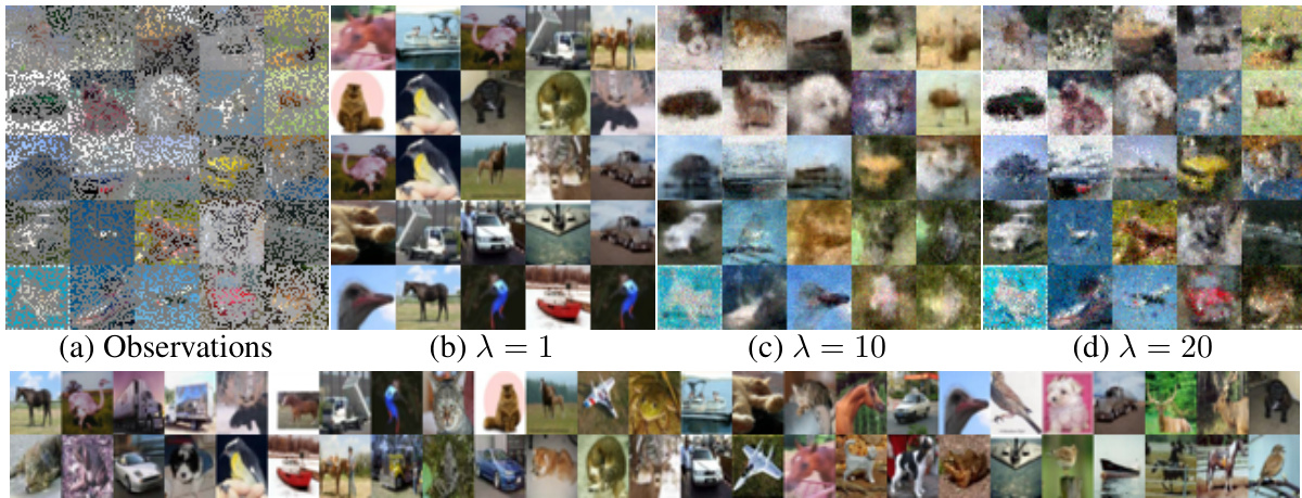
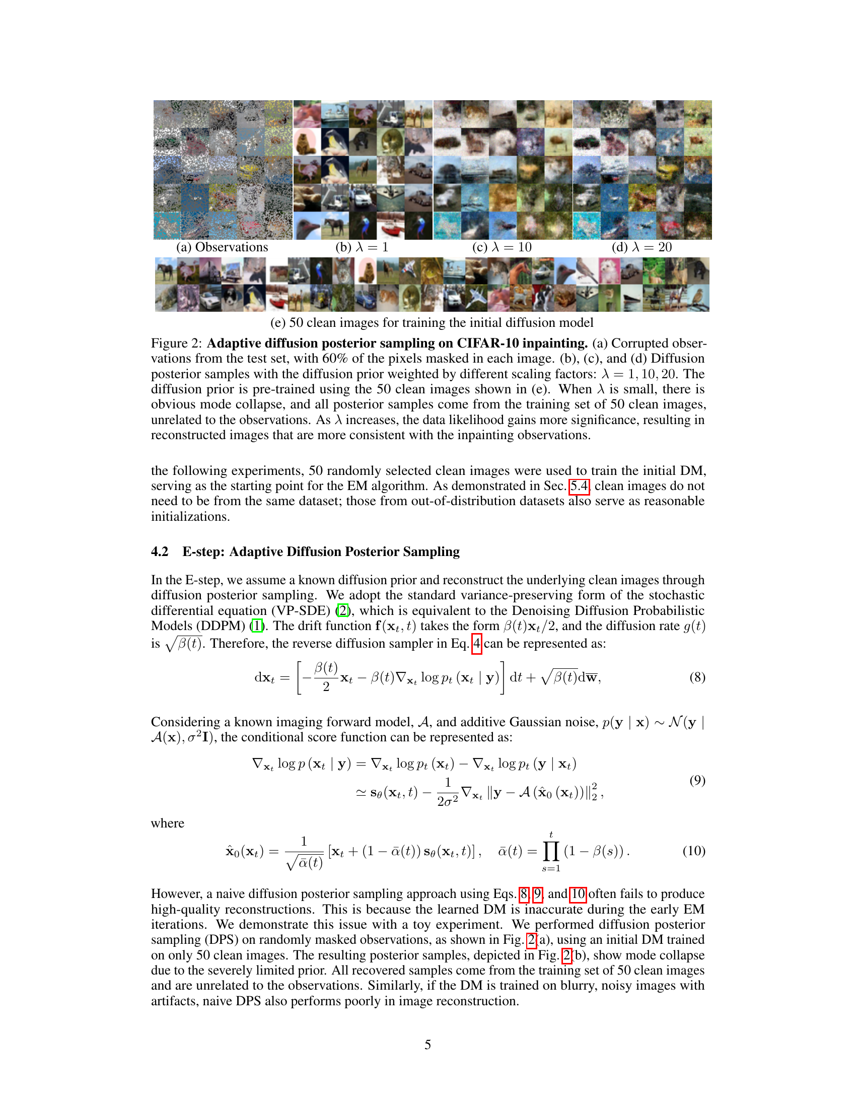
🔼 This figure shows the results of adaptive diffusion posterior sampling on CIFAR-10 inpainting. It demonstrates how the quality of posterior samples improves as the scaling factor (λ) increases, showing the effect of balancing the diffusion prior and data likelihood.
read the caption
Figure 2: Adaptive diffusion posterior sampling on CIFAR-10 inpainting. (a) Corrupted observations from the test set, with 60% of the pixels masked in each image. (b), (c), and (d) Diffusion posterior samples with the diffusion prior weighted by different scaling factors: λ = 1, 10, 20. The diffusion prior is pre-trained using the 50 clean images shown in (e). When λ is small, there is obvious mode collapse, and all posterior samples come from the training set of 50 clean images, unrelated to the observations. As λ increases, the data likelihood gains more significance, resulting in reconstructed images that are more consistent with the inpainting observations.
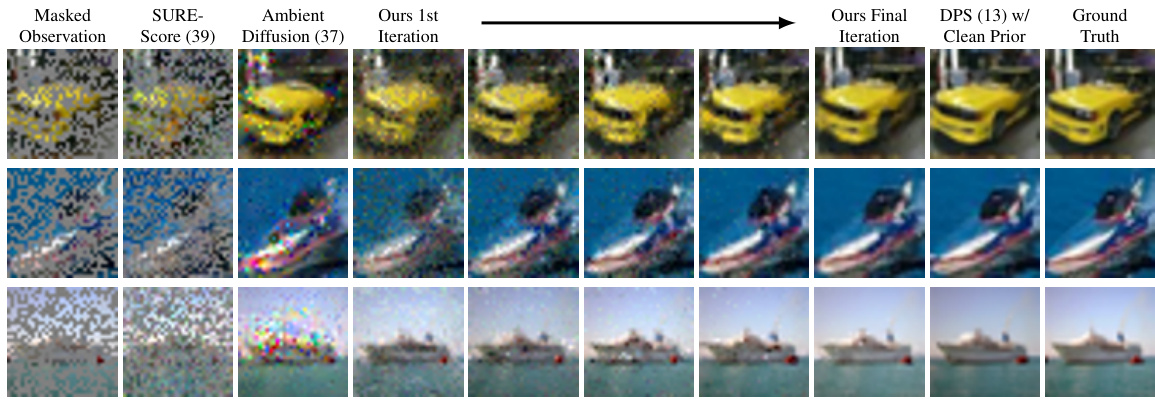
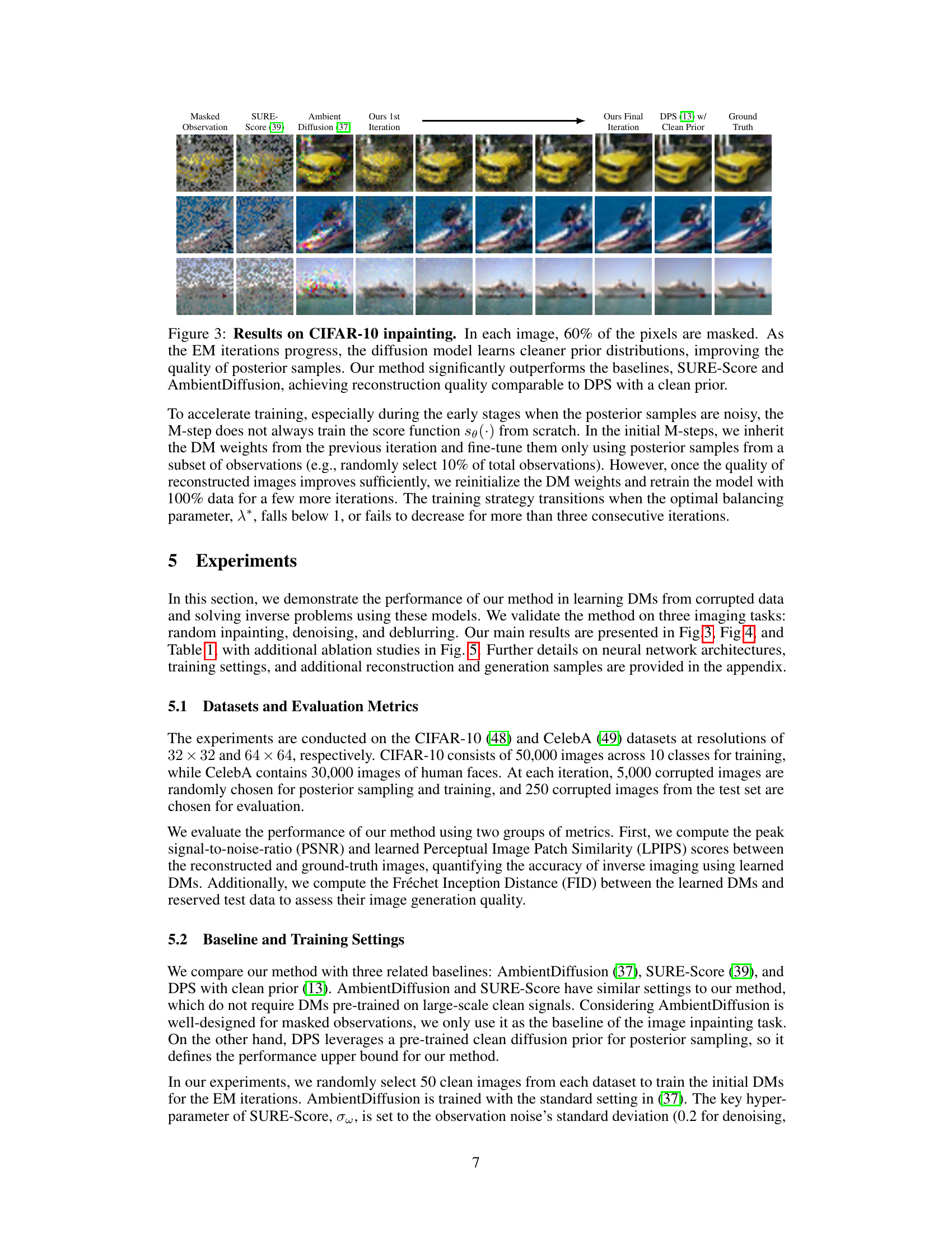
🔼 This figure shows the results of inpainting on CIFAR-10 dataset. 60% of the pixels are masked in each image. The results from different methods are shown, including SURE-Score, Ambient Diffusion, the proposed method at its first and final iterations, DPS with a clean prior, and the ground truth images. The figure demonstrates the iterative improvement of the proposed method’s inpainting quality through EM iterations and highlights its superior performance compared to existing baselines.
read the caption
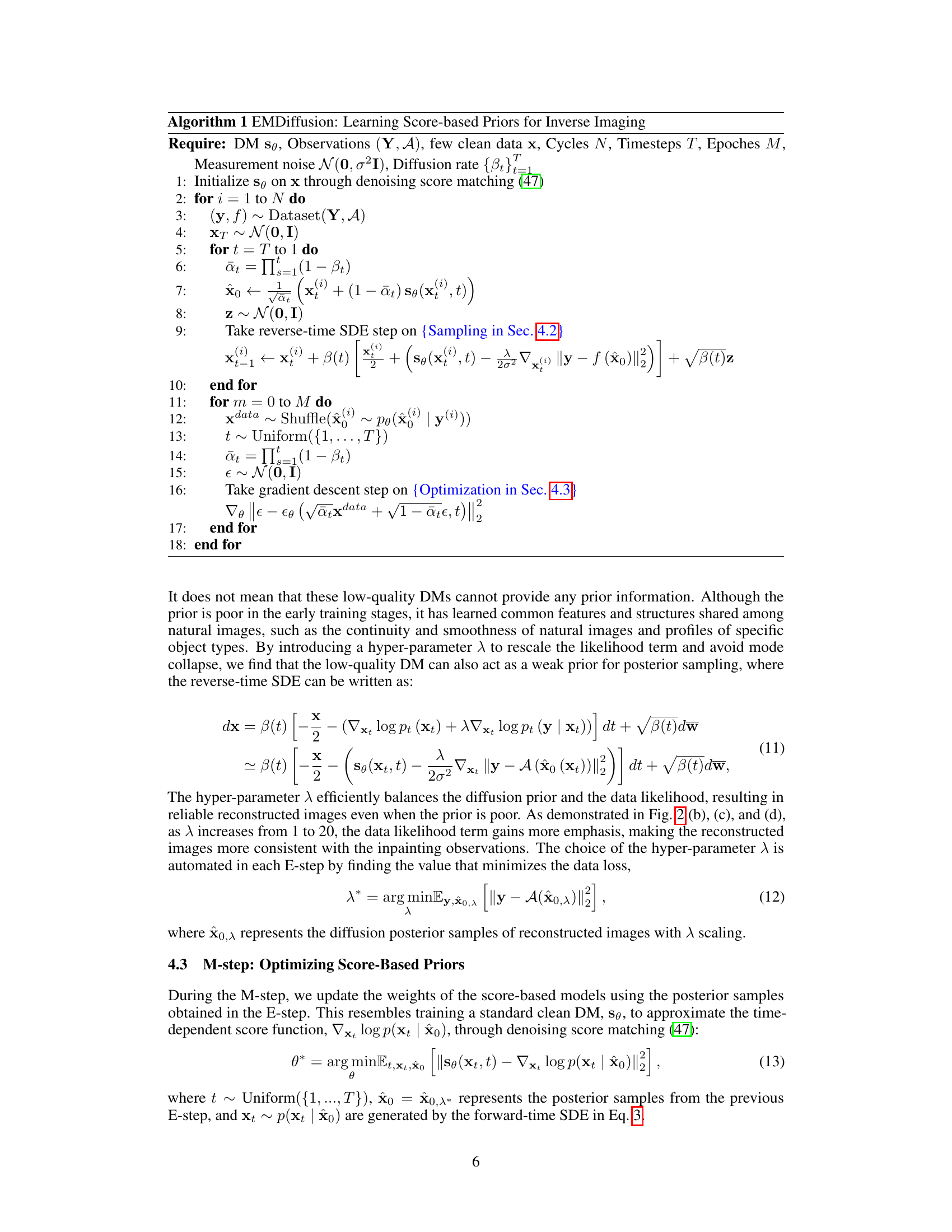
Figure 3: Results on CIFAR-10 inpainting. In each image, 60% of the pixels are masked. As the EM iterations progress, the diffusion model learns cleaner prior distributions, improving the quality of posterior samples. Our method significantly outperforms the baselines, SURE-Score and AmbientDiffusion, achieving reconstruction quality comparable to DPS with a clean prior.
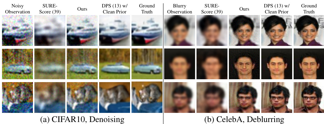
🔼 This figure shows the results of the proposed EMDiffusion method on CIFAR-10 image inpainting task, where 60% of the pixels are randomly masked in each image. It compares the results of EMDiffusion with those from two baseline methods (SURE-Score and AmbientDiffusion) and DPS (Diffusion Posterior Sampling) using a clean prior. The figure demonstrates that as the EM iterations progress, EMDiffusion produces progressively cleaner reconstructions, surpassing the baseline methods and achieving a quality similar to DPS with access to a clean training dataset.
read the caption
Figure 3: Results on CIFAR-10 inpainting. In each image, 60% of the pixels are masked. As the EM iterations progress, the diffusion model learns cleaner prior distributions, improving the quality of posterior samples. Our method significantly outperforms the baselines, SURE-Score and AmbientDiffusion, achieving reconstruction quality comparable to DPS with a clean prior.

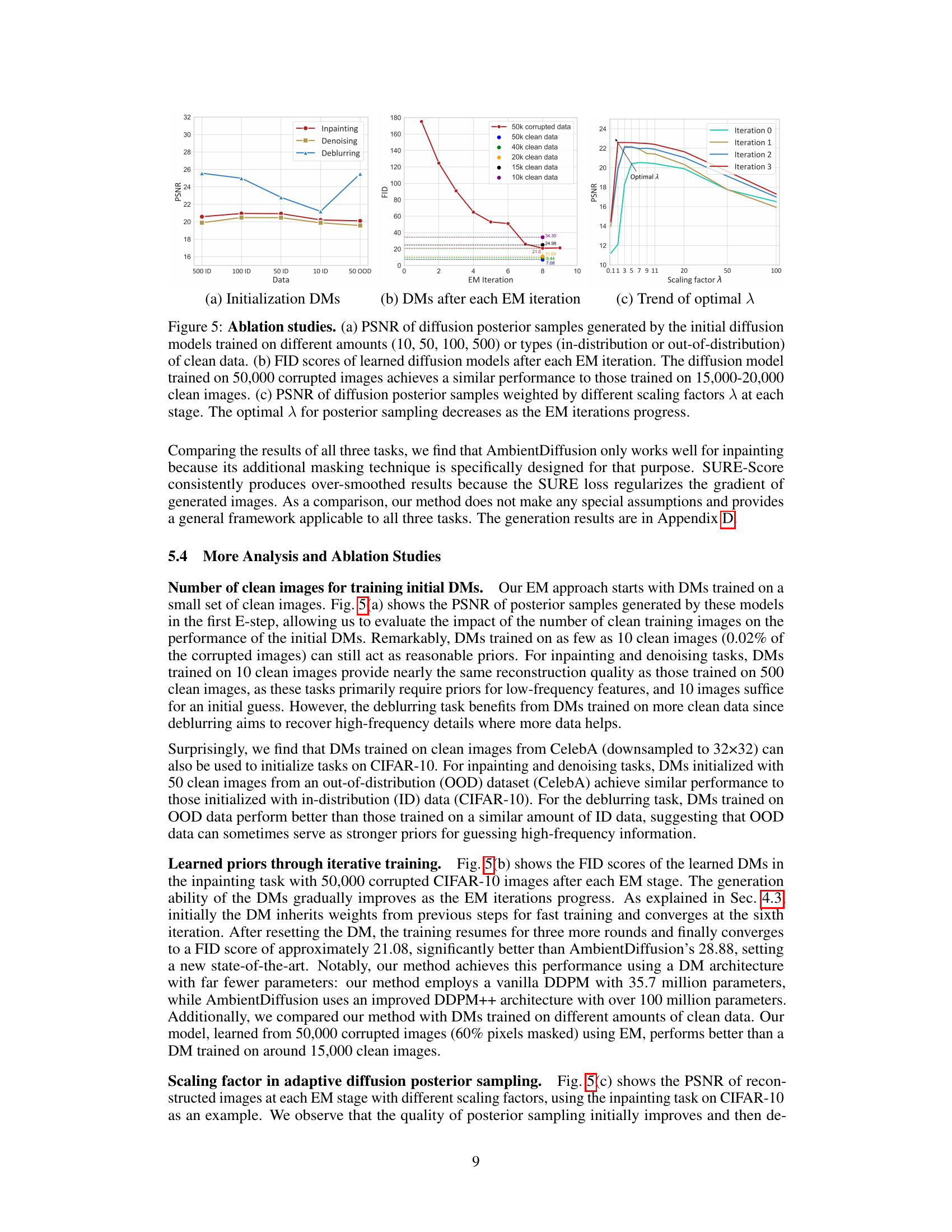
🔼 This figure presents ablation study results to analyze the impact of different factors on the performance of the proposed EMDiffusion method. Subfigure (a) shows how the quality of initial diffusion models varies depending on the number and source (in-distribution vs. out-of-distribution) of clean images used for training. Subfigure (b) illustrates the evolution of the FID score (a measure of generated image quality) for learned diffusion models across multiple EM iterations. Finally, subfigure (c) demonstrates how the optimal scaling factor (λ) for posterior sampling changes over EM iterations. The results demonstrate the robustness of the method to variations in the initialization, and its effectiveness in converging toward an optimal solution.
read the caption
Figure 5: Ablation studies. (a) PSNR of diffusion posterior samples generated by the initial diffusion models trained on different amounts (10, 50, 100, 500) or types (in-distribution or out-of-distribution) of clean data. (b) FID scores of learned diffusion models after each EM iteration. The diffusion model trained on 50,000 corrupted images achieves a similar performance to those trained on 15,000–20,000 clean images. (c) PSNR of diffusion posterior samples weighted by different scaling factors λ at each stage. The optimal λ for posterior sampling decreases as the EM iterations progress.

🔼 This figure compares the image inpainting results of the proposed EMDiffusion method against two baselines (SURE-Score and Ambient Diffusion) and a method using a clean diffusion prior (DPS). The figure shows that the proposed method significantly improves the image quality as the EM iterations progress, eventually achieving results comparable to the method with a clean prior, while significantly outperforming the baselines. Each image has 60% of its pixels masked.
read the caption
Figure 3: Results on CIFAR-10 inpainting. In each image, 60% of the pixels are masked. As the EM iterations progress, the diffusion model learns cleaner prior distributions, improving the quality of posterior samples. Our method significantly outperforms the baselines, SURE-Score and AmbientDiffusion, achieving reconstruction quality comparable to DPS with a clean prior.

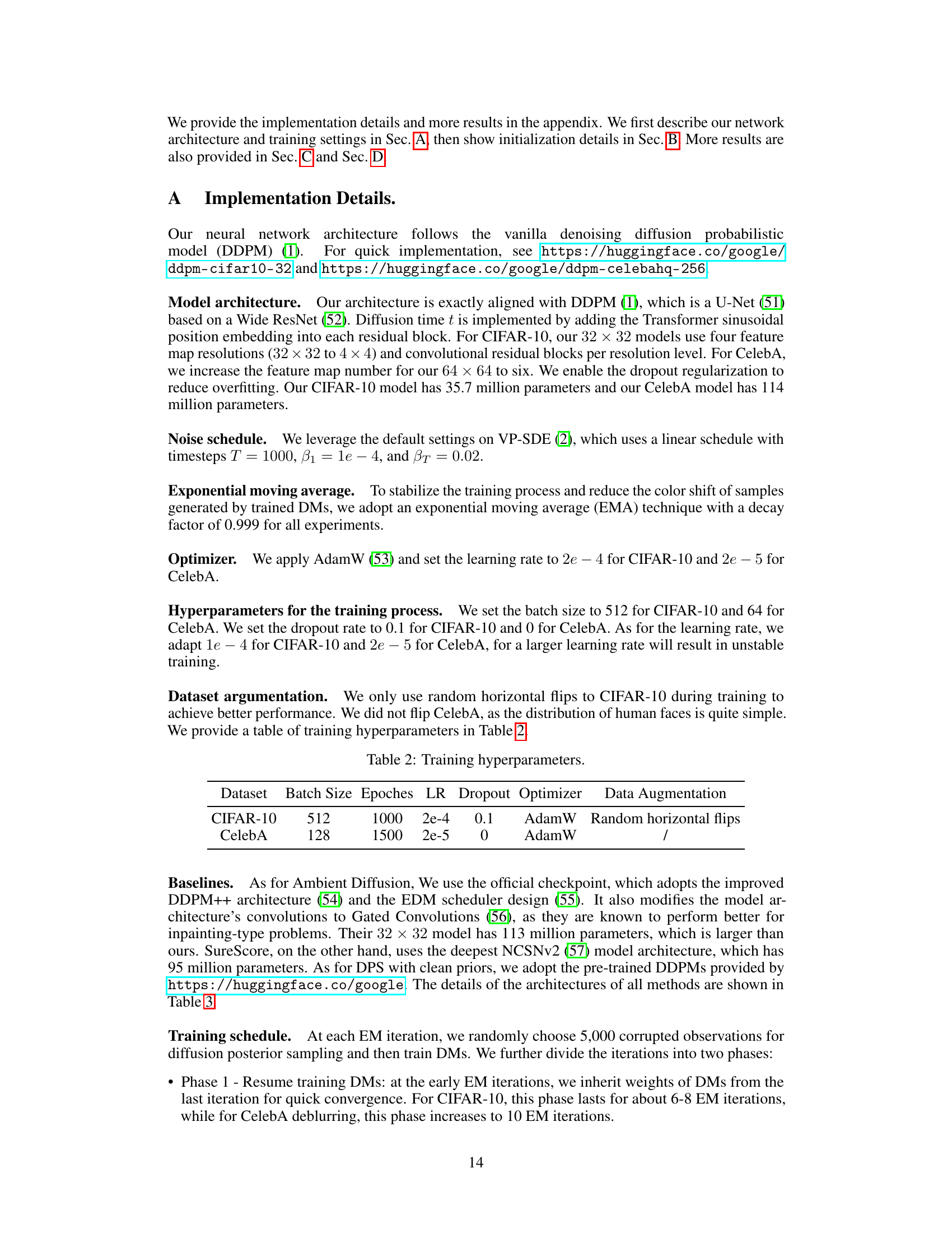
🔼 This figure shows samples generated by different models trained on blurry CelebA images. It compares the quality of generated images from SURE-Score (a), Ambient Diffusion (b), and the proposed EMDiffusion method (c). The FID (Fréchet Inception Distance) scores are provided for each model to quantitatively evaluate the quality of the generated samples. Lower FID scores indicate higher quality and better similarity to real images.
read the caption
Figure 6: Uncurated Samples generated from models trained on blurry CelebA.
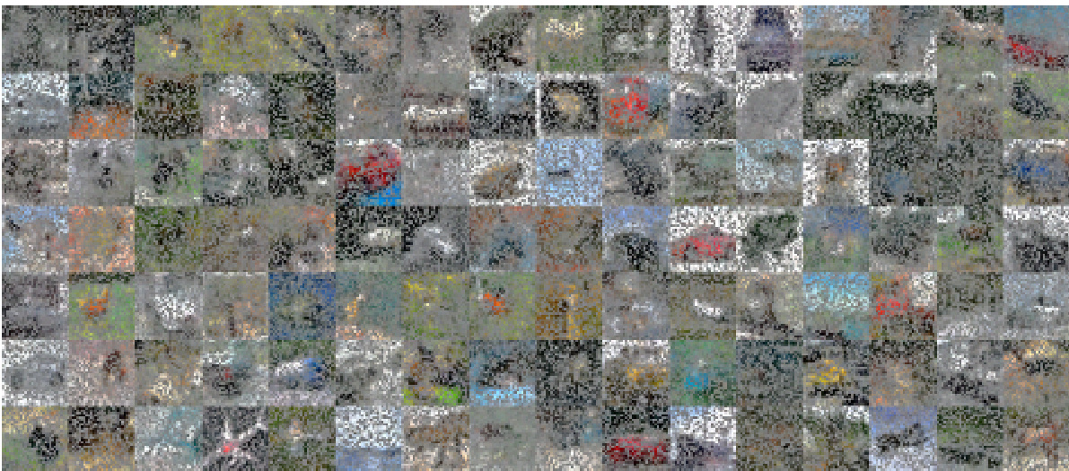
🔼 This figure shows the results of adaptive diffusion posterior sampling on CIFAR-10 inpainting. It demonstrates how changing the scaling factor (λ) affects the quality of the posterior samples generated from a diffusion model. With a small λ, the model collapses to the training data and ignores the observations. Increasing λ balances the prior and data likelihood, resulting in better reconstructions.
read the caption
Figure 2: Adaptive diffusion posterior sampling on CIFAR-10 inpainting. (a) Corrupted observations from the test set, with 60% of the pixels masked in each image. (b), (c), and (d) Diffusion posterior samples with the diffusion prior weighted by different scaling factors: λ = 1, 10, 20. The diffusion prior is pre-trained using the 50 clean images shown in (e). When λ is small, there is obvious mode collapse, and all posterior samples come from the training set of 50 clean images, unrelated to the observations. As λ increases, the data likelihood gains more significance, resulting in reconstructed images that are more consistent with the inpainting observations.
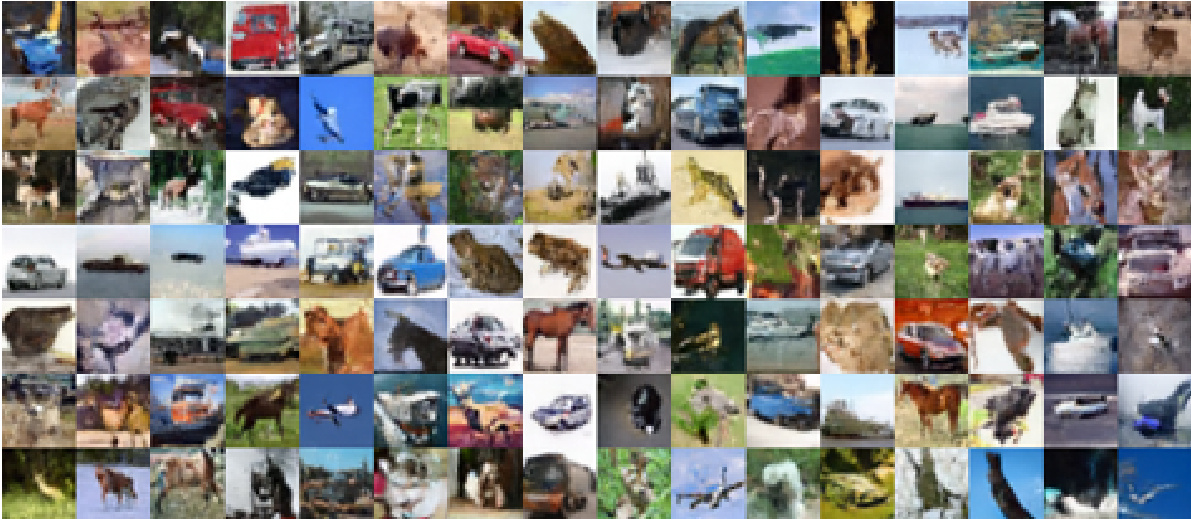
🔼 This figure shows the effect of the scaling factor (lambda) on the quality of the posterior samples generated by adaptive diffusion posterior sampling for image inpainting on the CIFAR-10 dataset. It demonstrates how a small lambda leads to mode collapse (samples resembling the training data, not the input), while increasing lambda improves sample quality, making them more consistent with the corrupted input images. The figure also shows the 50 clean images used to pre-train the initial diffusion model.
read the caption
Figure 2: Adaptive diffusion posterior sampling on CIFAR-10 inpainting. (a) Corrupted observations from the test set, with 60% of the pixels masked in each image. (b), (c), and (d) Diffusion posterior samples with the diffusion prior weighted by different scaling factors: A = 1, 10, 20. The diffusion prior is pre-trained using the 50 clean images shown in (e). When A is small, there is obvious mode collapse, and all posterior samples come from the training set of 50 clean images, unrelated to the observations. As A increases, the data likelihood gains more significance, resulting in reconstructed images that are more consistent with the inpainting observations.

🔼 This figure demonstrates the effect of the scaling factor λ in adaptive diffusion posterior sampling for image inpainting on the CIFAR-10 dataset. It shows that with a small λ, the model collapses to the training data and ignores the input, while increasing λ allows the model to better utilize the information in the corrupted input for reconstruction.
read the caption
Figure 2: Adaptive diffusion posterior sampling on CIFAR-10 inpainting. (a) Corrupted observations from the test set, with 60% of the pixels masked in each image. (b), (c), and (d) Diffusion posterior samples with the diffusion prior weighted by different scaling factors: λ = 1, 10, 20. The diffusion prior is pre-trained using the 50 clean images shown in (e). When λ is small, there is obvious mode collapse, and all posterior samples come from the training set of 50 clean images, unrelated to the observations. As λ increases, the data likelihood gains more significance, resulting in reconstructed images that are more consistent with the inpainting observations.

🔼 This figure shows the effect of scaling factor λ on the quality of posterior samples generated by adaptive diffusion posterior sampling for image inpainting on the CIFAR-10 dataset. It demonstrates how adjusting λ balances the influence of the pre-trained diffusion model (prior) and the observed data (likelihood), resulting in improved image reconstruction as λ increases and the data likelihood’s influence grows.
read the caption
Figure 2: Adaptive diffusion posterior sampling on CIFAR-10 inpainting. (a) Corrupted observations from the test set, with 60% of the pixels masked in each image. (b), (c), and (d) Diffusion posterior samples with the diffusion prior weighted by different scaling factors: A = 1, 10, 20. The diffusion prior is pre-trained using the 50 clean images shown in (e). When A is small, there is obvious mode collapse, and all posterior samples come from the training set of 50 clean images, unrelated to the observations. As A increases, the data likelihood gains more significance, resulting in reconstructed images that are more consistent with the inpainting observations.
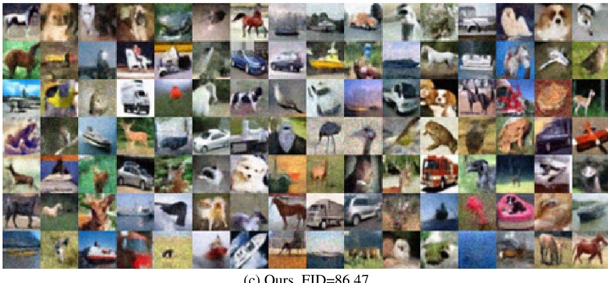
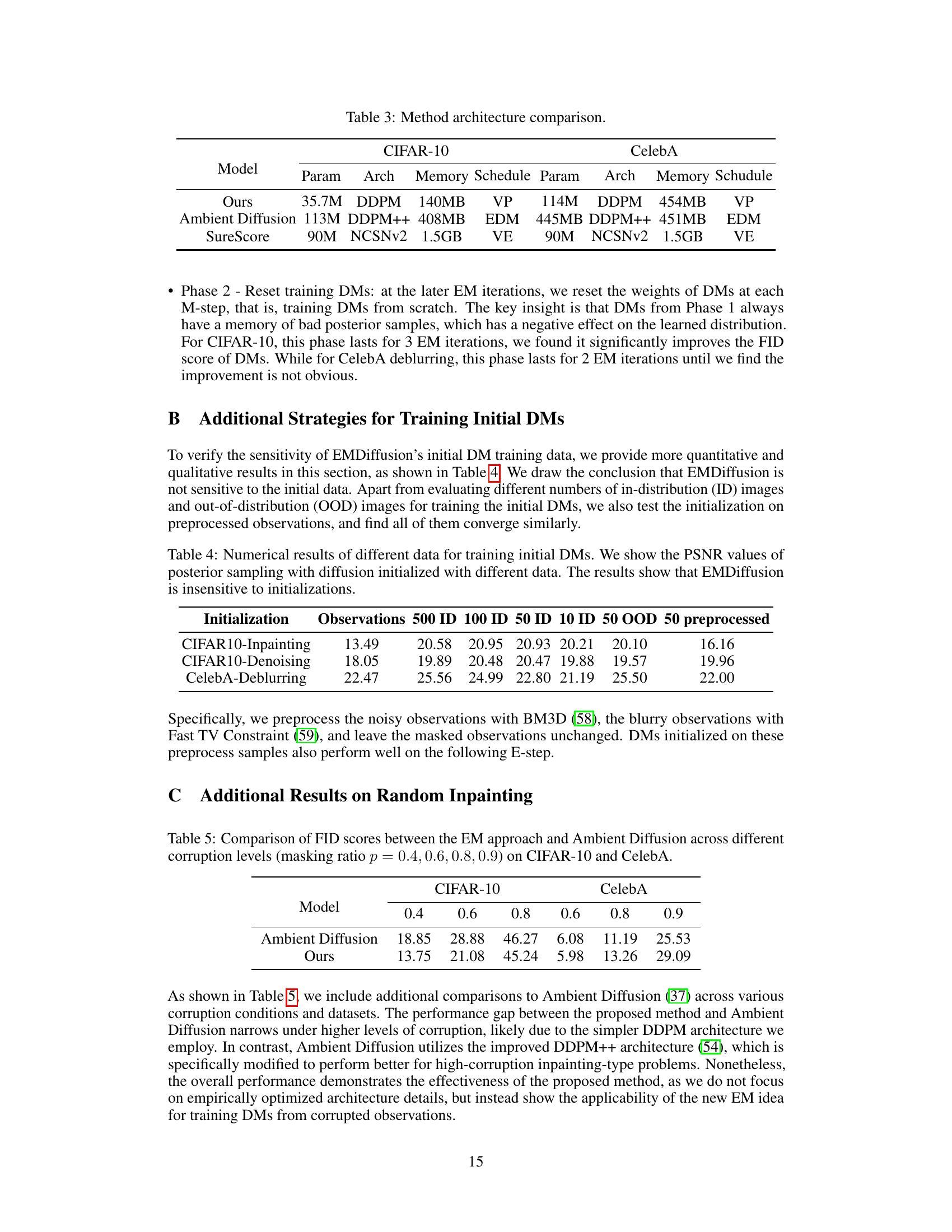
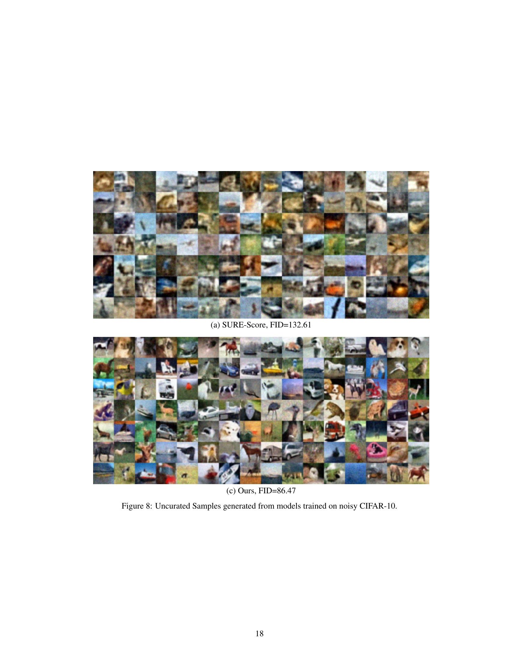
🔼 This figure displays 100 samples generated from diffusion models trained on noisy CIFAR-10 data. It visually demonstrates the quality of the generated images by the model. The FID score (Fréchet Inception Distance) is provided as a quantitative measure of the similarity between the generated samples and real CIFAR-10 images. A lower FID score indicates better image generation quality. This figure is used for comparison with other methods’ results, providing a visual assessment of the quality of image generation.
read the caption
Figure 8: Uncurated Samples generated from models trained on noisy CIFAR-10.
More on tables

🔼 This table presents a quantitative comparison of the proposed EMDiffusion method against several baselines on three inverse imaging tasks: inpainting, denoising, and deblurring. Performance is evaluated using Peak Signal-to-Noise Ratio (PSNR), Learned Perceptual Image Patch Similarity (LPIPS), and Fréchet Inception Distance (FID). Higher PSNR and lower LPIPS indicate better image reconstruction quality, while lower FID suggests the generated samples from the learned diffusion model are closer to the true data distribution. The results show that EMDiffusion significantly outperforms the baselines in most cases.
read the caption
Table 1: Numerical Results of inverse imaging and learned priors. The average values of PSNR/LPIPS are from 250 samples randomly selected from the test set. FID is used to evaluate the quality of learned priors by comparing 50,000 generated samples to the train set. Optimal results are highlighted in bold and suboptimal results in underline. Note that we take DPS w/ clean prior as the upper bound.

🔼 This table presents a comparison of different methods for inverse imaging tasks (inpainting, denoising, and deblurring) using various metrics: PSNR (Peak Signal-to-Noise Ratio), LPIPS (Learned Perceptual Image Patch Similarity), and FID (Fréchet Inception Distance). The table shows the performance of the proposed EMDiffusion method against baselines, including DPS (Diffusion Posterior Sampling) with a clean prior (representing an upper bound), and highlights the superior performance of EMDiffusion, particularly in achieving high PSNR and low LPIPS scores.
read the caption
Table 1: Numerical Results of inverse imaging and learned priors. The average values of PSNR/LPIPS are from 250 samples randomly selected from the test set. FID is used to evaluate the quality of learned priors by comparing 50,000 generated samples to the train set. Optimal results are highlighted in bold and suboptimal results in underline. Note that we take DPS w/ clean prior as the upper bound.

🔼 This table presents a quantitative comparison of different methods for inverse imaging problems, including the proposed EMDiffusion. It shows the Peak Signal-to-Noise Ratio (PSNR), Learned Perceptual Image Patch Similarity (LPIPS), and Fréchet Inception Distance (FID) scores for image inpainting, denoising, and deblurring tasks on CIFAR-10 and CelebA datasets. The results highlight EMDiffusion’s performance compared to baselines, using a clean prior as an upper bound for evaluation.
read the caption
Table 1: Numerical Results of inverse imaging and learned priors. The average values of PSNR/LPIPS are from 250 samples randomly selected from the test set. FID is used to evaluate the quality of learned priors by comparing 50,000 generated samples to the train set. Optimal results are highlighted in bold and suboptimal results in underline. Note that we take DPS w/ clean prior as the upper bound.

🔼 This table presents a quantitative comparison of different methods for inverse imaging tasks (inpainting, denoising, and deblurring) using learned diffusion models. The metrics used are Peak Signal-to-Noise Ratio (PSNR), Learned Perceptual Image Patch Similarity (LPIPS), and Fréchet Inception Distance (FID). PSNR and LPIPS assess reconstruction quality, while FID evaluates the quality of the learned prior distribution by comparing generated images to real images. The table shows that the proposed method achieves state-of-the-art performance, as indicated by the bolded values.
read the caption
Table 1: Numerical Results of inverse imaging and learned priors. The average values of PSNR/LPIPS are from 250 samples randomly selected from the test set. FID is used to evaluate the quality of learned priors by comparing 50,000 generated samples to the train set. Optimal results are highlighted in bold and suboptimal results in underline. Note that we take DPS w/ clean prior as the upper bound.
Full paper#
