TL;DR#
Many real-world datasets contain multiple distributions that have shifted due to changes in their underlying causal mechanisms. Existing methods for causal representation learning (CRL) require interventions on each latent factor and data from many environments. This requirement is very difficult to satisfy. This creates challenges in identifying the sources of distribution shifts.
This paper introduces a novel approach that addresses this limitation. It introduces a new algorithm that identifies the latent factors that are responsible for the distribution shifts using a limited number of coarsely measured interventions. The algorithm is scalable and can be applied to datasets with a high number of latent variables. The authors demonstrate that their approach works well on both synthetic and real-world datasets.
Key Takeaways#
Why does it matter?#
This paper is crucial because it tackles a key challenge in causal representation learning: identifying the root causes of distribution shifts in complex systems with limited interventional data. Its novel identifiability results and algorithm are highly valuable for researchers working with high-dimensional data and complex causal structures, opening new avenues for causal discovery and root cause analysis across various fields.
Visual Insights#

🔼 This figure illustrates an example of the problem setting with 5 latent variables representing personality traits. Observed data (X) comes from a psychometric test with 50 questions. Three environments (US, UK, AU) are shown, each representing a different set of interventions on the latent variables. The goal is to identify the latent variables (Z) whose causal mechanisms have shifted between environments, based on observed changes in the distribution of X.
read the caption
Figure 1: We have 5 latent variables Z which in this case relate to personality concepts, and the observations X represent the scores of 50 questions from a psychometric personality test. The latent variables Z follow a linear SCM, while the unknown shared linear mixing is a full-rank matrix G∈ R50×5. Then, for environment k = {US, UK, AU}, the observables are generated through X(k) = GZ(k). Here, P(US) is taken as the “observational” (reference) distribution, and the distribution shifts in [P(UK) and [][P(AU) are due to changes in the causal mechanisms of {Z1} and {Z2, Z3, Z5}, respectively. Finally, the types of interventions are general; for UK, the edge Z4 → Z1 is removed and the dashed red lines indicate changes in the edge weights to Z₁; for AU, Z2 was intervened by removing Z5 → Z2 and adding Z3 → Z2, while the edge Z5 → Z3 was reversed, thus changing the mechanisms of Z3 and Z5. Thus, we aim to identify {Z1} and {Z2, Z3, Z5}.
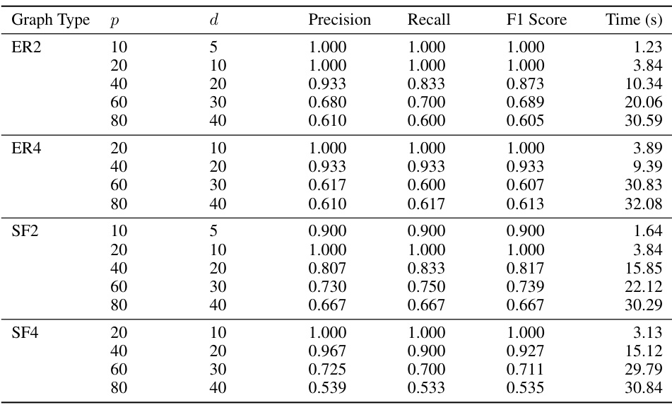
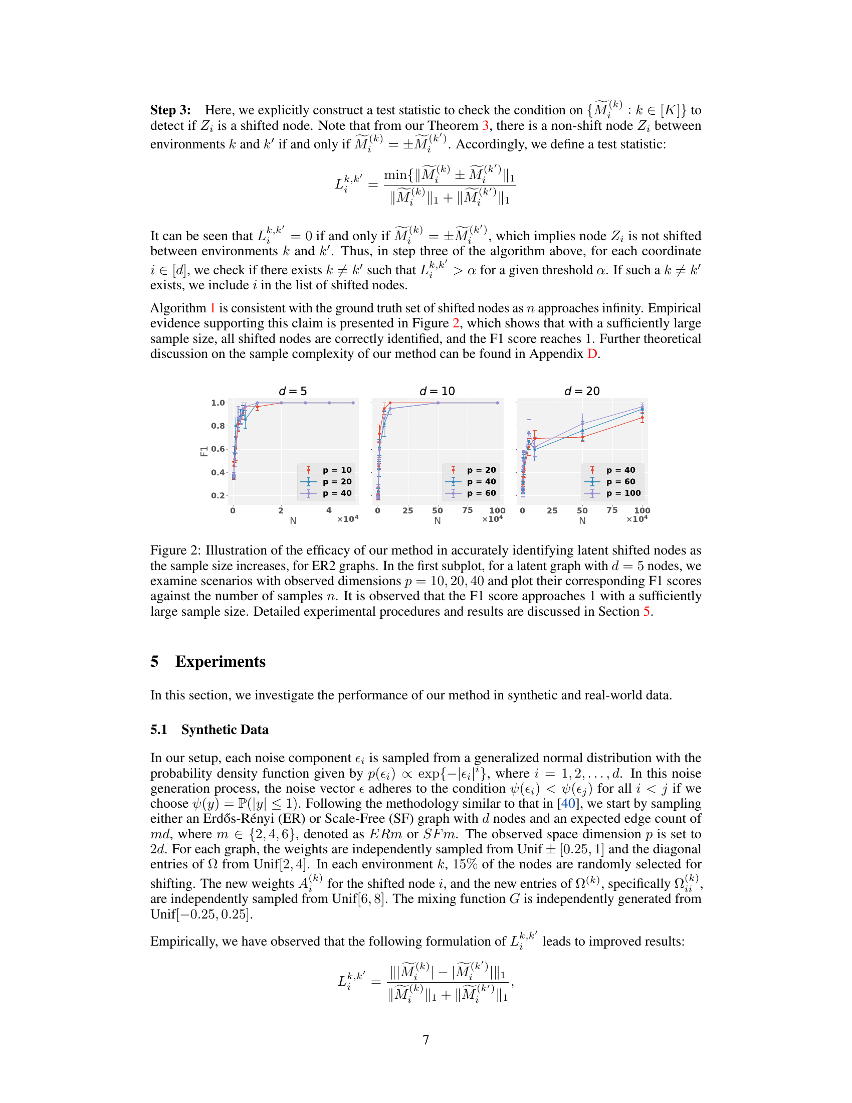
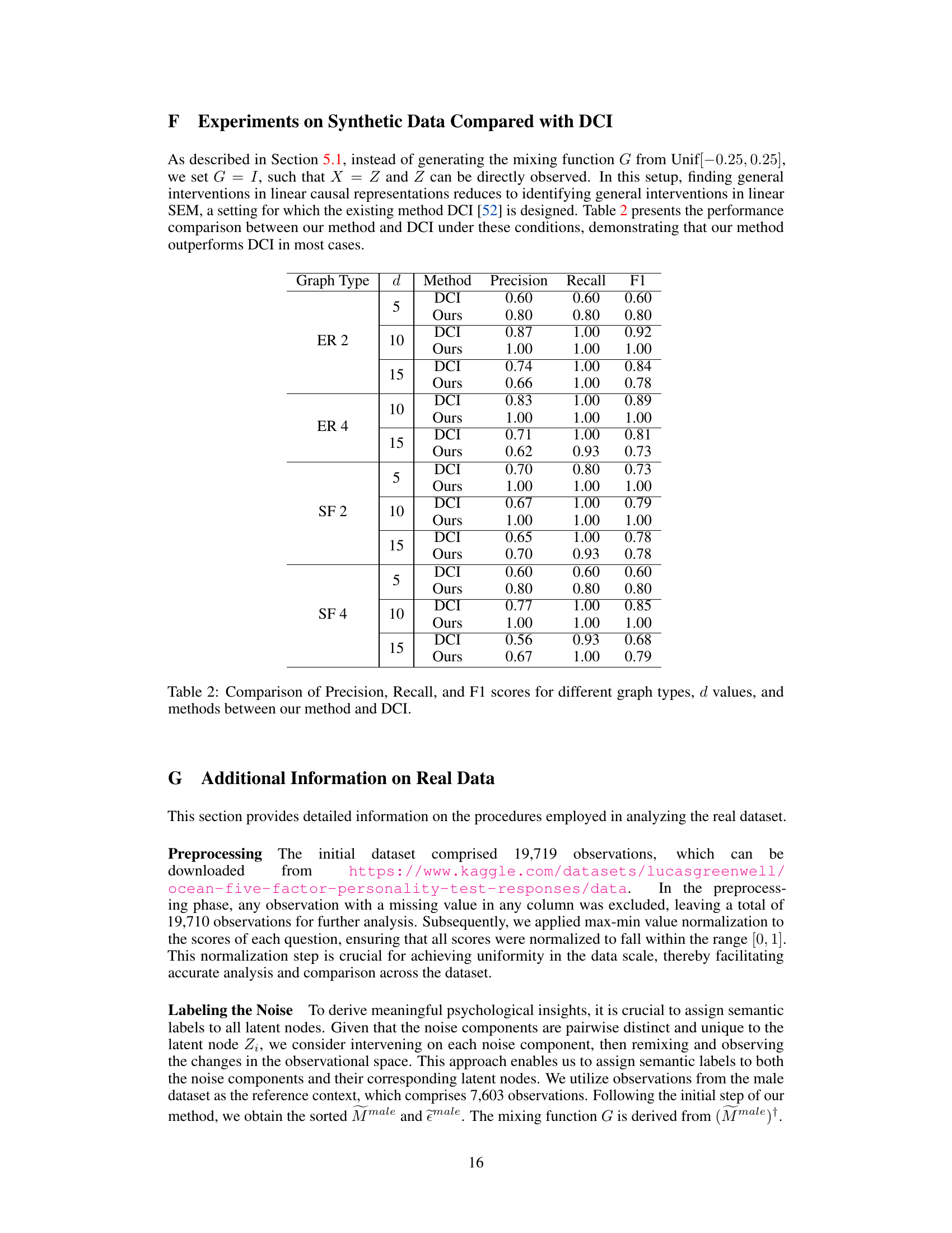
🔼 This table presents the results of experiments on synthetic data to evaluate the performance of the proposed method in identifying latent shifted nodes. It shows precision, recall, F1 score, and computation time for various graph types (ER2, ER4, SF2, SF4), dimensions (d), and observed dimensions (p). The results demonstrate the effectiveness of the method across different settings and sample sizes.
read the caption
Table 1: Performance metrics for shifted node detection across various graph configurations, sample sizes n
In-depth insights#
Mechanism Shift ID#
Mechanism Shift ID, in the context of causal representation learning, presents a significant challenge: identifying which latent causal factors have undergone changes across different environments or interventions. Successful identification hinges on disentangling the effects of confounding factors and intervention variations, enabling precise localization of the causal shifts. This requires moving beyond simple statistical discrepancy measures and leveraging the structure of the causal model to pinpoint shifts in conditional distributions rather than just marginal ones. A robust approach must account for various intervention types – from precise single-node manipulations to broader, more nuanced interventions that can drastically alter the underlying causal graph. This necessitates methods capable of handling incomplete or imperfect interventional data, and the ability to distinguish between actual causal shifts and spurious correlations caused by confounding factors or observation noise. The development of computationally efficient and statistically sound algorithms for Mechanism Shift ID remains a crucial area of research in causal inference, particularly when addressing high-dimensional data and complex causal relationships.
Linear Causal CRL#
Linear Causal Causal Representation Learning (CRL) focuses on uncovering causal relationships within data where latent variables, not directly observed, influence the observed variables. Linearity in this context assumes linear relationships between latent factors and both each other (via a structural causal model, SCM) and the observed variables. This simplifies the mathematical framework, making it more tractable than nonlinear models. However, this simplification limits its applicability to systems where such linearity truly holds. A key advantage of linear causal CRL is identifiability: under certain conditions (sufficient interventions, etc.), the underlying causal structure and latent variables can be recovered up to certain ambiguities (like scaling or ordering of variables). This identifiability, however, often depends on assumptions about the nature and number of interventions available. The need for interventions is a practical limitation, as in many real-world scenarios perfectly controlled interventions might be impossible or very difficult to implement. Future research will likely explore more robust methods that handle non-linearity, fewer interventions, or noisy data. Despite these limitations, linear causal CRL provides a foundational framework for understanding causal mechanisms in complex systems, particularly where linear approximations offer a reasonable degree of accuracy.
ICA for Shift Detection#
Independent Component Analysis (ICA) offers a powerful approach for shift detection by leveraging its ability to separate mixed signals into independent components. In the context of shift detection, ICA can isolate the sources of variation in data, identifying which components exhibit significant changes across different datasets or time points. This is particularly valuable when dealing with high-dimensional data where direct observation of individual shifts is challenging. By decomposing the observed data into its constituent components, ICA provides a structured representation suitable for identifying and quantifying these changes. The independence assumption of ICA is crucial, as it enables the disentanglement of overlapping signals, ensuring that the detected shifts are not artifacts of signal mixing. However, limitations exist. The performance of ICA is sensitive to the non-Gaussianity of the source signals, and assumptions about independence may not always hold in real-world scenarios. Moreover, ICA’s ability to accurately identify shifts depends on sufficient data and the nature of the shifts themselves. Despite these challenges, the application of ICA for shift detection offers a potentially robust and informative means of understanding the sources of data changes in complex systems.
Psychometric Dataset#
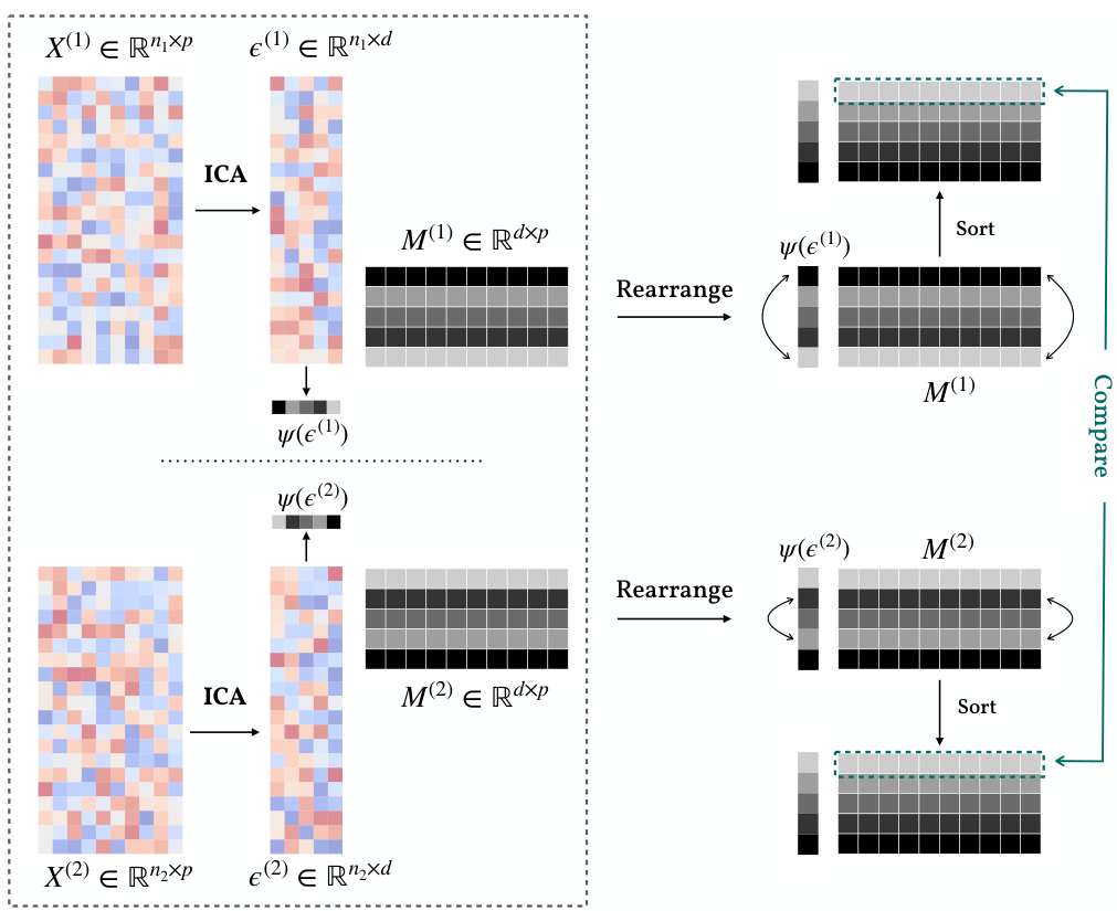
The study leverages a psychometric dataset to evaluate its method in a real-world scenario. The dataset contains responses from participants to personality questionnaires, measuring the Big Five personality traits (Openness, Conscientiousness, Extraversion, Agreeableness, Neuroticism). This provides a rich environment to assess the model’s ability to identify latent personality dimensions and changes across different groups. By focusing on gender and nationality comparisons (US vs. UK), the researchers aim to identify latent personality shifts. The choice of this dataset is particularly insightful because it allows for the validation of the method’s findings against existing psychological literature on gender and cross-cultural personality differences. This is important because it connects the computational results to a substantial body of existing knowledge, adding another layer of validation to the approach. The results of applying the method to the dataset are crucial in demonstrating the method’s practical applicability and providing a real-world context for its functionality.
Future Work: Non-linear#
Extending the research to non-linear causal relationships presents a significant and exciting challenge. Nonlinearity is ubiquitous in real-world phenomena, and linear models often fail to capture the complexity of these systems. The current identifiability results, which rely heavily on linearity, would require substantial re-evaluation. This necessitates developing new mathematical techniques and algorithms that can handle non-linear mixing functions and causal structures. A key difficulty will involve defining suitable analogs for intervention effects within a nonlinear framework. The theoretical analysis might involve tools from differential geometry or topology, depending on the type of nonlinearity considered. Furthermore, developing computationally efficient and scalable algorithms for this problem would pose a significant practical hurdle. Exploring specific types of non-linearity, such as those with additive noise or those that satisfy particular smoothness constraints, might offer a more manageable entry point. Ultimately, successfully addressing the non-linear case would greatly enhance the applicability and impact of the approach, opening the door to a broader range of causal discovery problems in diverse fields.
More visual insights#
More on figures

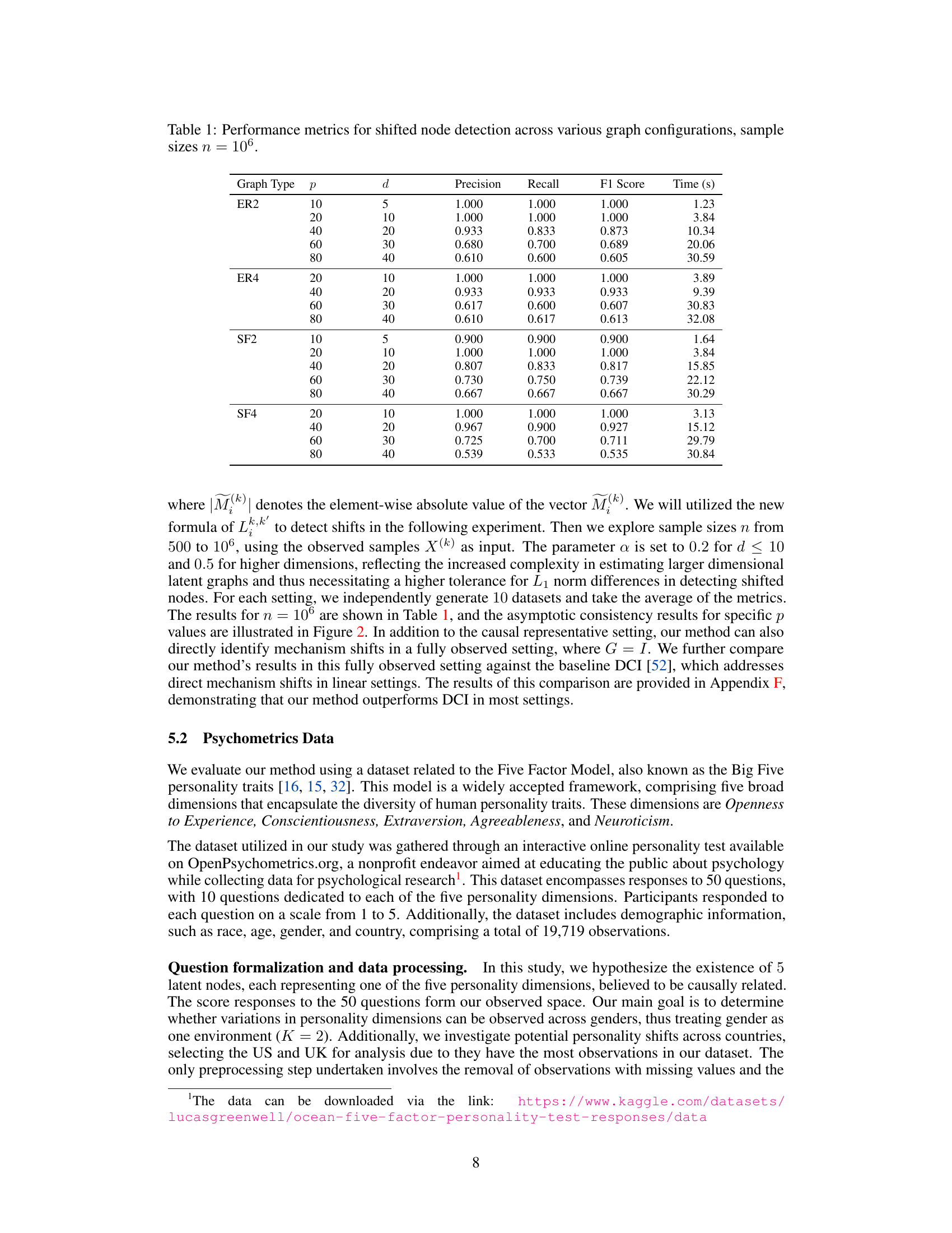
🔼 This figure shows the performance of the proposed method in identifying latent shifted nodes in synthetic data with varying sample sizes (N) and observed dimensions (p). The results demonstrate that the F1 score, a measure of the method’s accuracy, increases and approaches 1 as the sample size increases, for different graph types (ER2).
read the caption
Figure 2: Illustration of the efficacy of our method in accurately identifying latent shifted nodes as the sample size increases, for ER2 graphs. In the first subplot, for a latent graph with d = 5 nodes, we examine scenarios with observed dimensions p = 10, 20, 40 and plot their corresponding F1 scores against the number of samples n. It is observed that the F1 score approaches 1 with a sufficiently large sample size. Detailed experimental procedures and results are discussed in Section 5.

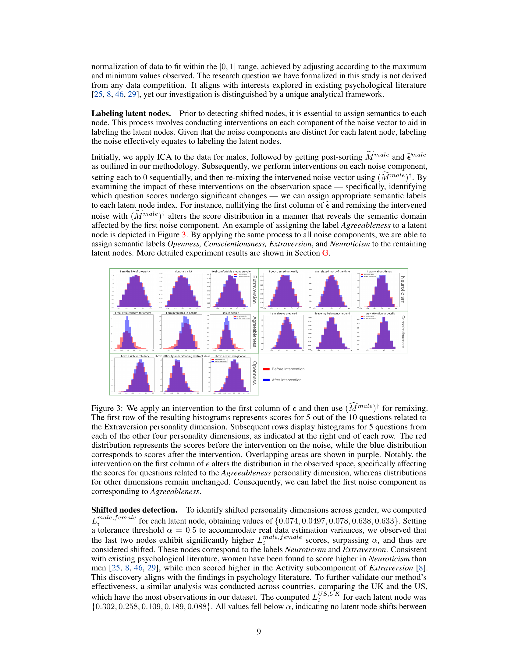
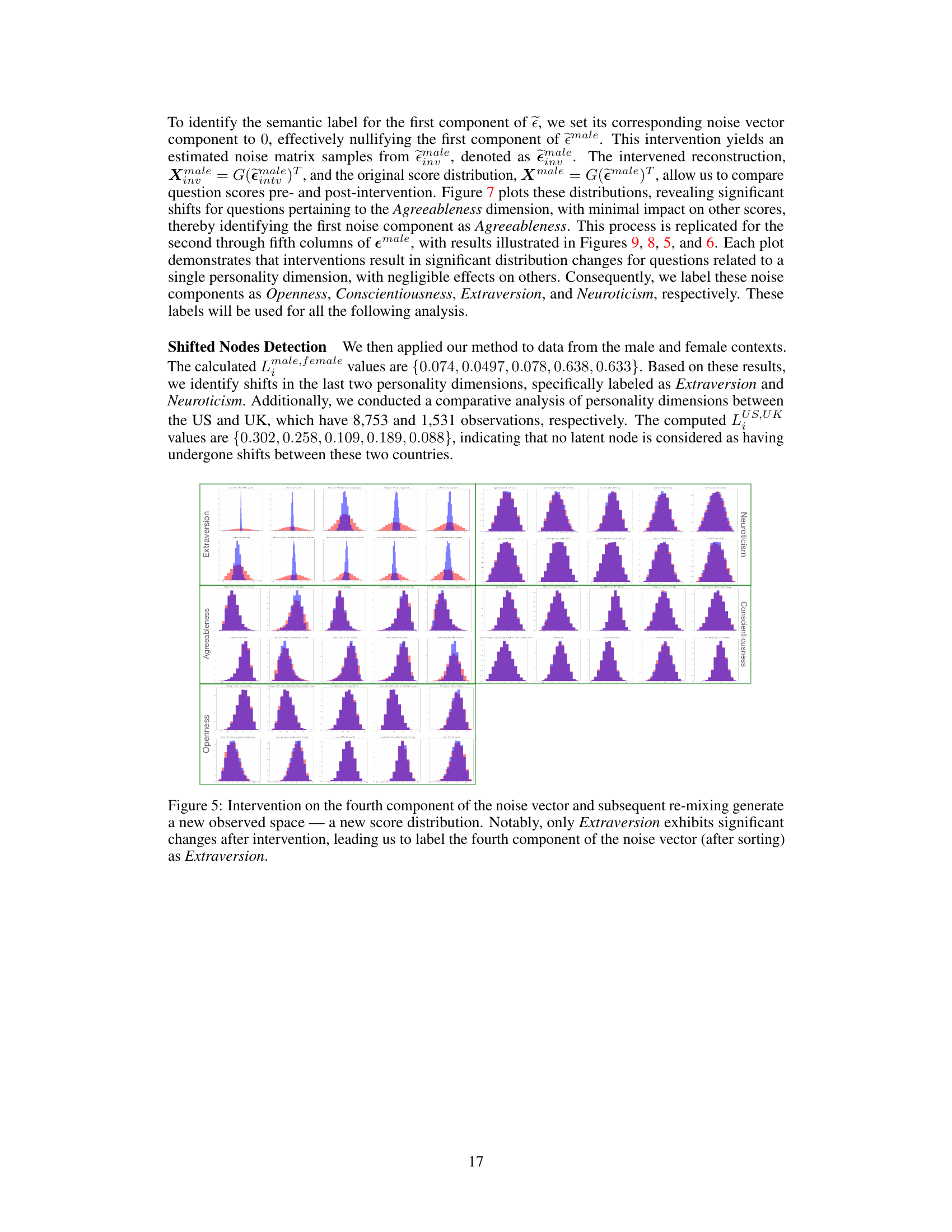
🔼 This figure shows the results of applying an intervention to the first component of the noise vector in the male dataset and remixing using the pseudoinverse of the mixing matrix. It illustrates how the intervention specifically affects the distribution of scores for questions related to the Agreeableness personality trait while leaving the scores for questions related to other personality traits largely unchanged. This observation allows the researchers to label the first noise component as corresponding to Agreeableness. The figure uses histograms to visualize the distributions before and after intervention for each of the five personality traits: Extraversion, Agreeableness, Conscientiousness, Neuroticism, and Openness.
read the caption
Figure 3: We apply an intervention to the first column of ϵ and then use (Mmale)† for remixing. The first row of the resulting histograms represents scores for 5 out of the 10 questions related to the Extraversion personality dimension. Subsequent rows display histograms for 5 questions from each of the other four personality dimensions, as indicated at the right end of each row. The red distribution represents the scores before the intervention on the noise, while the blue distribution corresponds to scores after the intervention. Overlapping areas are shown in purple. Notably, the intervention on the first column of e alters the distribution in the observed space, specifically affecting the scores for questions related to the Agreeableness personality dimension, whereas distributions for other dimensions remain unchanged. Consequently, we can label the first noise component as corresponding to Agreeableness.
🔼 This figure illustrates an example of the problem setting with 5 latent variables representing personality traits and 50 observed variables representing scores on personality test questions. Three different environments (US, UK, Australia) are shown, each with a slightly different causal structure between the latent variables. The goal is to identify which latent variables (Z1, Z2, Z3, Z4, Z5) have experienced changes in their causal mechanisms across the different environments. The figure highlights that changes can involve edge removals, additions, and weight changes. The observed variables (X) are a linear mixing of the latent variables.
read the caption
Figure 1: We have 5 latent variables Z which in this case relate to personality concepts, and the observations X represent the scores of 50 questions from a psychometric personality test. The latent variables Z follow a linear SCM, while the unknown shared linear mixing is a full-rank matrix G∈ R50×5. Then, for environment k = {US, UK, AU}, the observables are generated through X(k) = GZ(k). Here, P(US) is taken as the “observational” (reference) distribution, and the distribution shifts in [P(UK) and [][P(AU) are due to changes in the causal mechanisms of {Z1} and {Z2, Z3, Z5}, respectively. Finally, the types of interventions are general; for UK, the edge Z4 → Z1 is removed and the dashed red lines indicate changes in the edge weights to Z₁; for AU, Z2 was intervened by removing Z5 → Z2 and adding Z3 → Z2, while the edge Z5 → Z3 was reversed, thus changing the mechanisms of Z3 and Z5. Thus, we aim to identify {Z1} and {Z2, Z3, Z5}.
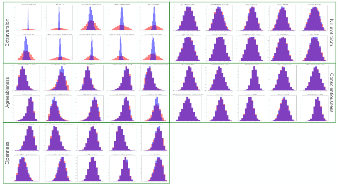
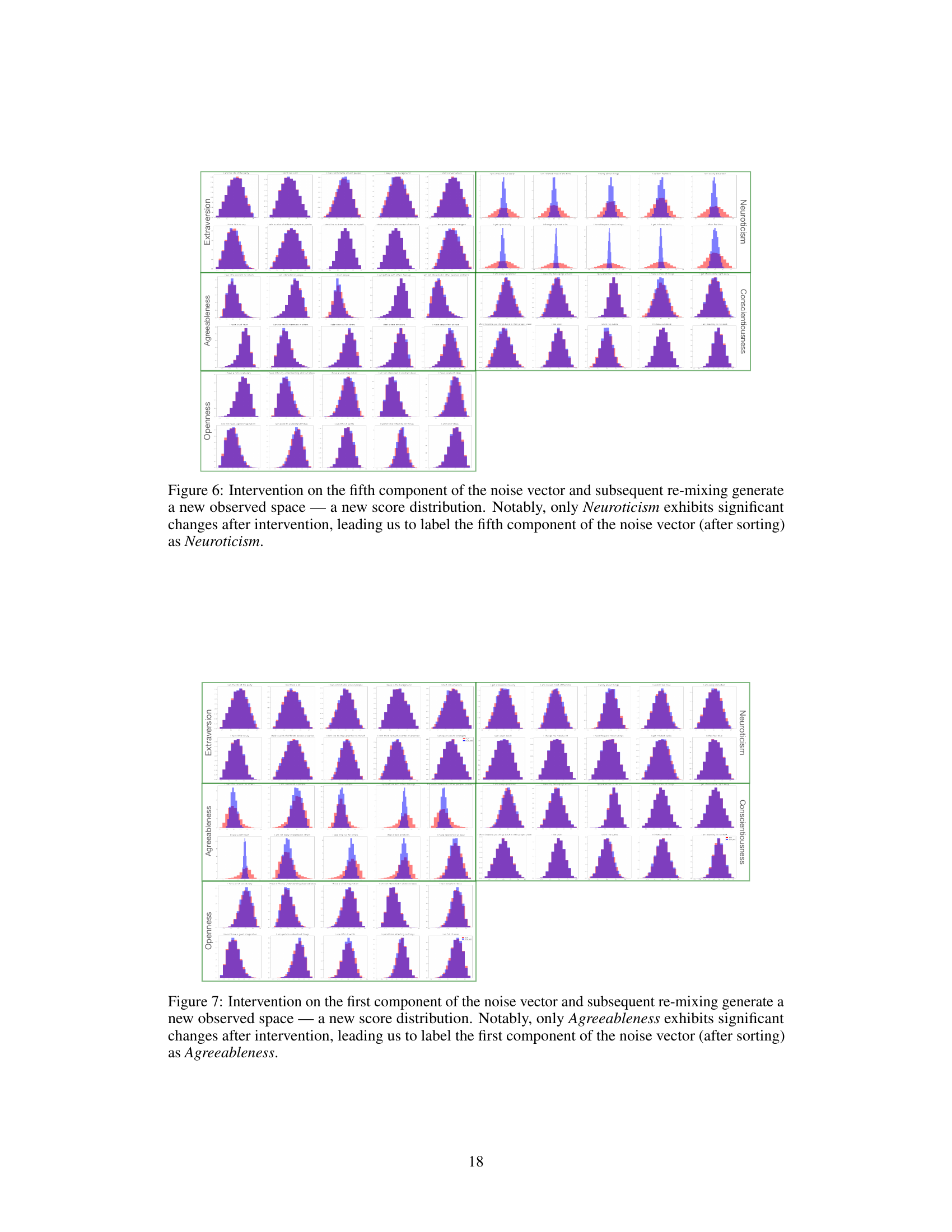
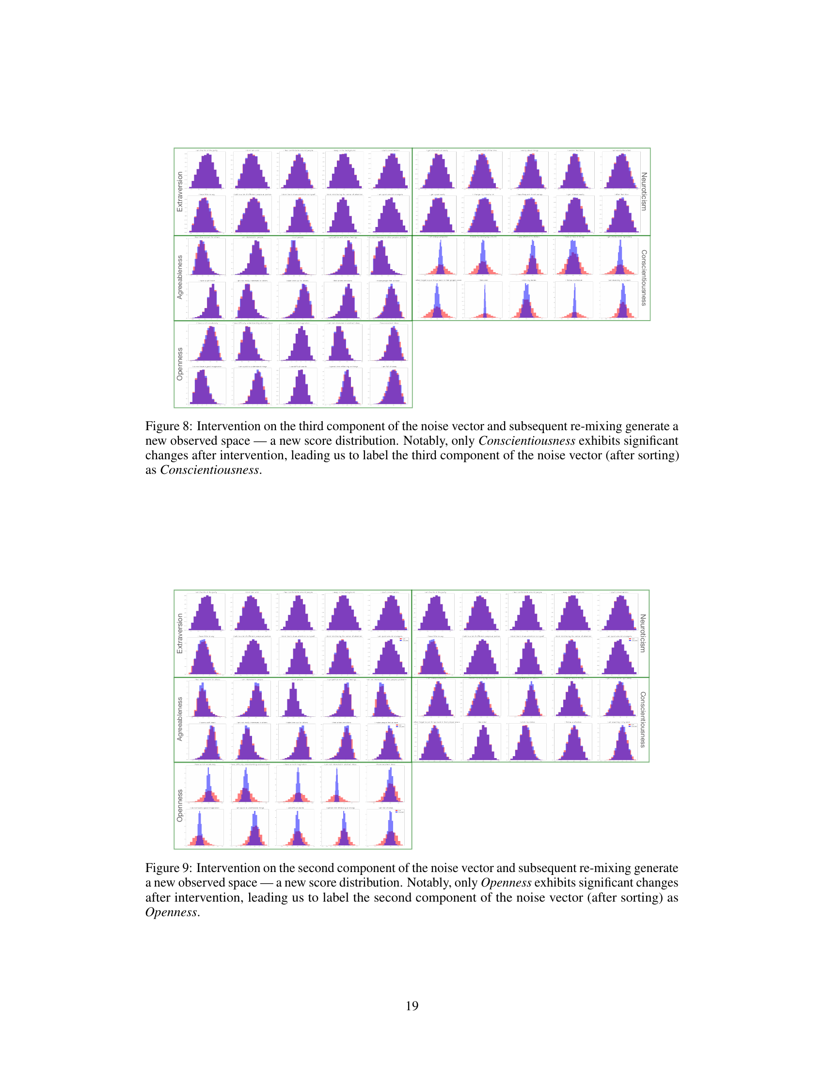
🔼 This figure shows the results of an intervention on the first component of the noise vector in the male dataset. Histograms display the distributions of scores for questions related to each of the Big Five personality traits before and after the intervention. The significant shift in the distribution of Agreeableness-related questions after the intervention on the first noise component allows for the labeling of that component as representing Agreeableness. This process is repeated for each noise component to label all five latent nodes.
read the caption
Figure 3: We apply an intervention to the first column of \(\epsilon\) and then use \((M^{\text{male}})^\dagger\) for remixing. The first row of the resulting histograms represents scores for 5 out of the 10 questions related to the Extraversion personality dimension. Subsequent rows display histograms for 5 questions from each of the other four personality dimensions, as indicated at the right end of each row. The red distribution represents the scores before the intervention on the noise, while the blue distribution corresponds to scores after the intervention. Overlapping areas are shown in purple. Notably, the intervention on the first column of \(\epsilon\) alters the distribution in the observed space, specifically affecting the scores for questions related to the Agreeableness personality dimension, whereas distributions for other dimensions remain unchanged. Consequently, we can label the first noise component as corresponding to Agreeableness.
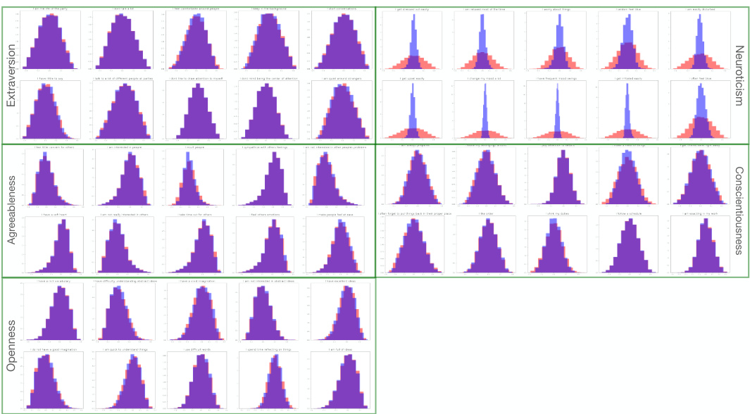
🔼 This figure shows the results of applying an intervention to the first component of the noise vector in a psychometric dataset. Histograms compare the distributions of question scores before and after the intervention. The significant shift in distributions related to Agreeableness questions demonstrates that the first noise component corresponds to this personality trait. This process is repeated for other noise components to label the remaining personality dimensions.
read the caption
Figure 3: We apply an intervention to the first column of and then use (Mmale)† for remixing. The first row of the resulting histograms represents scores for 5 out of the 10 questions related to the Extraversion personality dimension. Subsequent rows display histograms for 5 questions from each of the other four personality dimensions, as indicated at the right end of each row. The red distribution represents the scores before the intervention on the noise, while the blue distribution corresponds to scores after the intervention. Overlapping areas are shown in purple. Notably, the intervention on the first column of alters the distribution in the observed space, specifically affecting the scores for questions related to the Agreeableness personality dimension, whereas distributions for other dimensions remain unchanged. Consequently, we can label the first noise component as corresponding to Agreeableness.
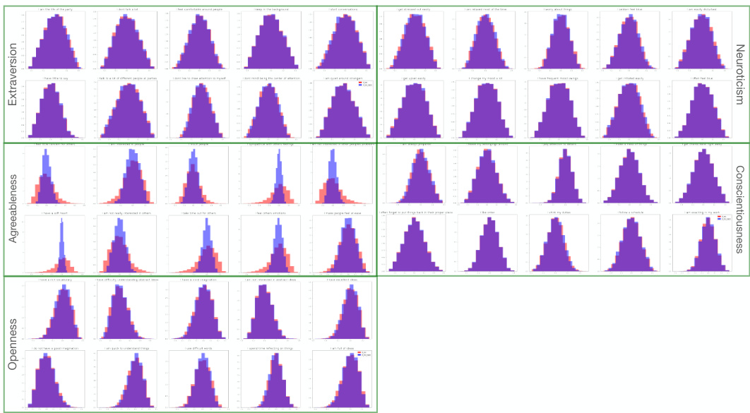
🔼 This figure shows the results of an intervention on the first component of the noise vector in the Big Five personality dataset. Histograms display the distributions of scores for questions related to each of the five personality traits (Extraversion, Agreeableness, Conscientiousness, Neuroticism, and Openness) before and after the intervention. The change in distribution for Agreeableness questions, while other traits remain largely unaffected, allows the researchers to label the first noise component as representing Agreeableness.
read the caption
Figure 3: We apply an intervention to the first column of and then use (Mmale)† for remixing. The first row of the resulting histograms represents scores for 5 out of the 10 questions related to the Extraversion personality dimension. Subsequent rows display histograms for 5 questions from each of the other four personality dimensions, as indicated at the right end of each row. The red distribution represents the scores before the intervention on the noise, while the blue distribution corresponds to scores after the intervention. Overlapping areas are shown in purple. Notably, the intervention on the first column of alters the distribution in the observed space, specifically affecting the scores for questions related to the Agreeableness personality dimension, whereas distributions for other dimensions remain unchanged. Consequently, we can label the first noise component as corresponding to Agreeableness.

🔼 This figure demonstrates how interventions on the noise components can be used to assign semantic labels to latent nodes. The figure shows the impact of nullifying the first noise component (related to Agreeableness) on the distribution of responses to questions in a psychometric personality test. The change in distribution for questions related to Agreeableness, while other dimensions remain unaffected, demonstrates how this technique helps label the latent nodes.
read the caption
Figure 3: We apply an intervention to the first column of \(\epsilon\) and then use \((M^{\text{male}})^\dagger\) for remixing. The first row of the resulting histograms represents scores for 5 out of the 10 questions related to the Extraversion personality dimension. Subsequent rows display histograms for 5 questions from each of the other four personality dimensions, as indicated at the right end of each row. The red distribution represents the scores before the intervention on the noise, while the blue distribution corresponds to scores after the intervention. Overlapping areas are shown in purple. Notably, the intervention on the first column of \(\epsilon\) alters the distribution in the observed space, specifically affecting the scores for questions related to the Agreeableness personality dimension, whereas distributions for other dimensions remain unchanged. Consequently, we can label the first noise component as corresponding to Agreeableness.

🔼 This figure shows the results of an intervention on the first component of the noise vector in the psychometric dataset. Histograms are shown to illustrate how the intervention changes the distribution of scores related to questions from each personality dimension (Extraversion, Neuroticism, Agreeableness, Conscientiousness, Openness). The figure demonstrates that intervening on the first noise component primarily affects the Agreeableness scores while leaving other dimensions largely unaffected, supporting the labeling of the first noise component as Agreeableness.
read the caption
Figure 3: We apply an intervention to the first column of ϵ and then use (Mmale)† for remixing. The first row of the resulting histograms represents scores for 5 out of the 10 questions related to the Extraversion personality dimension. Subsequent rows display histograms for 5 questions from each of the other four personality dimensions, as indicated at the right end of each row. The red distribution represents the scores before the intervention on the noise, while the blue distribution corresponds to scores after the intervention. Overlapping areas are shown in purple. Notably, the intervention on the first column of ϵ alters the distribution in the observed space, specifically affecting the scores for questions related to the Agreeableness personality dimension, whereas distributions for other dimensions remain unchanged. Consequently, we can label the first noise component as corresponding to Agreeableness.
Full paper#
