Near-Minimax-Optimal Distributional Reinforcement Learning with a Generative Model

↗ OpenReview ↗ NeurIPS Homepage ↗ Chat

TL;DR

#

Key Takeaways

#

Why does it matter?

#

This paper is crucial for researchers in reinforcement learning as it bridges the gap between theoretical lower bounds and practical algorithms for distributional reinforcement learning, offering a near-minimax optimal algorithm and new theoretical insights for categorical approaches. This opens doors for improved sample efficiency in various applications and inspires further research on tractable algorithms and new distributional Bellman equations.

Visual Insights

#

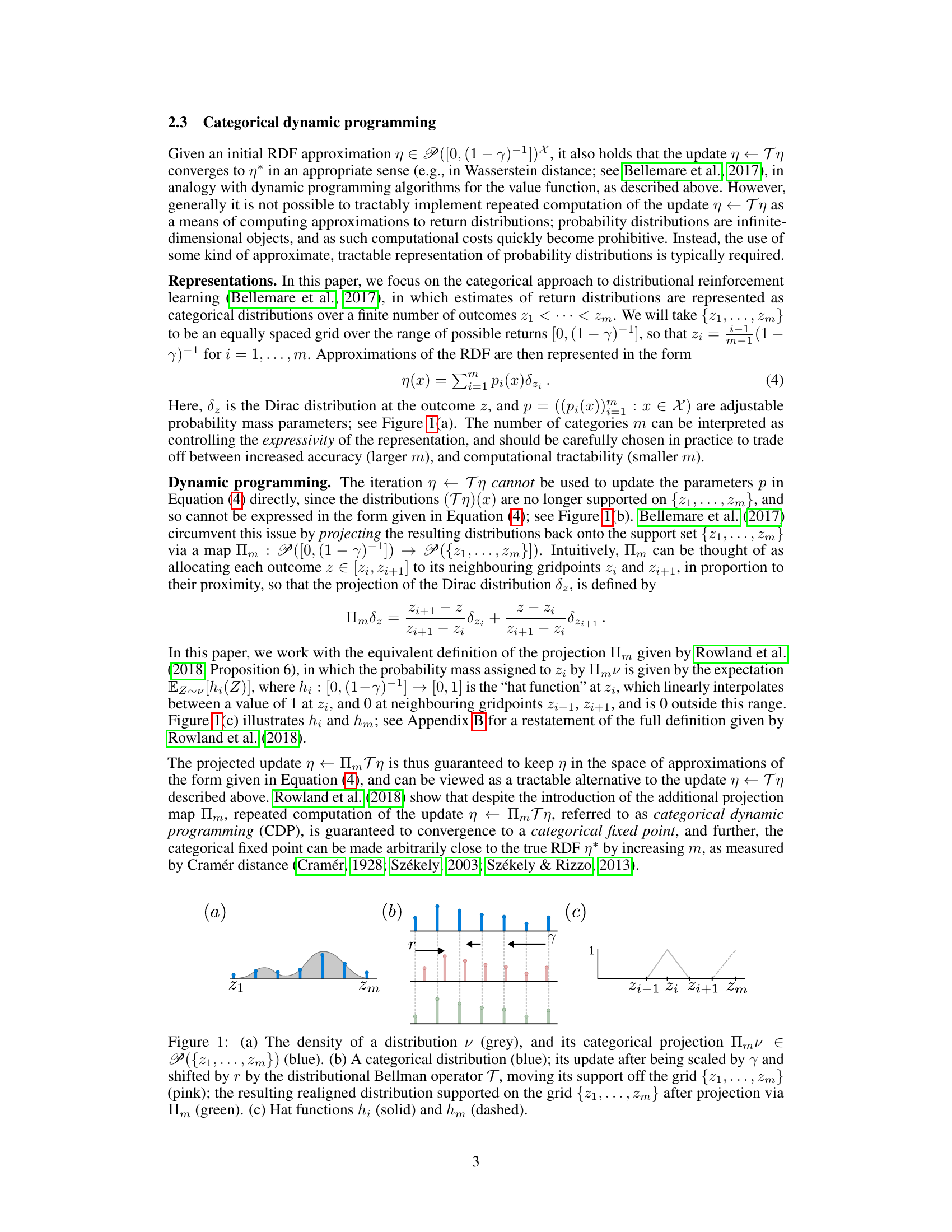
This figure illustrates the categorical dynamic programming approach to distributional reinforcement learning. Panel (a) shows how a continuous distribution is projected onto a discrete set of points, representing a categorical distribution. Panel (b) demonstrates the distributional Bellman update, which shifts and scales the categorical distribution, causing its support to fall outside the original grid. A projection step is then required to map the updated distribution back onto the grid, as shown in the figure. Panel (c) shows the hat functions used to perform this projection.

This figure compares the performance of various distributional reinforcement learning algorithms (DCFP, QDP, CDP) across different settings. The x-axis represents either the number of samples per state or wall-clock time, and the y-axis shows the approximation error (Wasserstein distance). Different plots show the results for varying discount factors (γ), numbers of atoms (m), and algorithms.

In-depth insights

#

Minimax Optimality

#

The concept of ‘Minimax Optimality’ in a machine learning context, especially within reinforcement learning, signifies achieving the best performance under the worst-case scenario. It’s a robust approach focusing on minimizing the maximum possible loss or regret, thereby guaranteeing a certain level of performance regardless of the specific circumstances or adversary’s actions. In the provided research paper, proving minimax optimality for a distributional reinforcement learning algorithm is a significant contribution. This implies the algorithm’s performance is guaranteed to be close to the theoretically best possible, even when facing an environment exhibiting the highest degree of uncertainty or adversarial behavior. This result is particularly powerful due to the inherent challenges of distributional reinforcement learning, where the goal is to estimate the full distribution of future rewards, rather than just their expected value. Demonstrating minimax optimality implies not only efficacy but also a strong theoretical guarantee of the algorithm’s efficiency and resilience against unpredictable factors in the learning process. The research likely leverages techniques from game theory and statistical learning to obtain this result, which is a considerable advancement in the theoretical understanding of distributional RL.

DCFP Algorithm

#

The Direct Categorical Fixed-Point (DCFP) algorithm presents a novel approach to distributional reinforcement learning, directly computing the categorical fixed point instead of iterative approximations. This offers significant computational advantages, especially when dealing with large state spaces. The algorithm’s core strength lies in its near-minimax optimality, meaning it achieves a sample complexity matching theoretical lower bounds, making it highly sample-efficient. This efficiency is crucial in model-based RL, where accurate distribution estimation relies heavily on the availability of sufficient data from a generative model. The theoretical foundation is robust, employing a novel stochastic categorical CDF Bellman equation to analyze the algorithm’s convergence. However, despite its theoretical strengths, the algorithm’s practical performance can be affected by factors such as environment stochasticity and discount factor, highlighting the need for careful consideration during implementation.

Categorical CDP

#

Categorical CDP, a distributional reinforcement learning algorithm, tackles the challenge of approximating return distributions using a computationally tractable approach. It overcomes the limitations of directly representing infinite-dimensional probability distributions by using categorical representations, essentially discretizing the distribution into a finite number of bins or categories. This approximation allows for efficient implementation of the distributional Bellman operator, which updates the return distribution estimates. The algorithm’s effectiveness depends on the number of categories used, trading off accuracy against computational cost. A key aspect of categorical CDP is the projection step, which maps the updated (often non-categorical) distribution back onto the categorical support, ensuring the algorithm’s convergence and numerical tractability. While the approximation limits accuracy, the algorithm is theoretically sound and has been proven to converge to the true return distribution under specific conditions. The choice of the number of categories and the projection method significantly impact both the accuracy and computational efficiency of the algorithm, therefore presenting a trade-off that needs careful consideration in practical applications.

Empirical Evaluation

#

An empirical evaluation section in a research paper is crucial for validating theoretical claims. It should present results comparing the proposed method to established baselines, using diverse datasets and metrics. Detailed methodology outlining data splits, hyperparameters, and evaluation protocols is essential for reproducibility. The analysis should include error bars and statistical tests to demonstrate significance and robustness. Visualizations like plots and tables should be clear, well-labeled, and easy to interpret, showing trends and highlighting key differences between approaches. A discussion of results is needed, explaining observed phenomena, addressing limitations, and exploring potential future work directions. A strong empirical evaluation section builds confidence in the paper’s contributions and helps readers understand the practical implications of the research.

Future Directions

#

Future research could explore several promising avenues. Extending the theoretical analysis to other distributional RL algorithms, such as quantile dynamic programming, would provide a more comprehensive understanding of their sample complexities. Investigating the impact of different distributional representations on the efficiency and accuracy of these algorithms is crucial. Developing more sophisticated methods for handling the complexities of high-dimensional state and action spaces is also necessary for practical applications. The paper mentions the possibility of using sparse linear solvers for improved efficiency; a deeper investigation into these methods and their scalability is warranted. Furthermore, the impact of environment stochasticity and discount factors on algorithm performance requires more in-depth analysis. Combining distributional RL with other advanced techniques, such as model-based reinforcement learning, could yield even greater improvements in sample efficiency and performance. Finally, applying the developed techniques to real-world problems, particularly in domains such as robotics, healthcare, and algorithm discovery, will be critical for demonstrating practical value.

More visual insights

#

More on figures

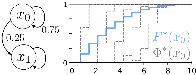
The left panel shows a simple Markov Reward Process with two states (x0 and x1) and a discount factor of 0.9. The reward is 1 for state x0 and 0 for state x1. The right panel shows the CDF of the categorical fixed point (blue line), generated by solving the equation: F = TpF (Equation (10) in the paper), and 5 independent samples from the stochastic categorical CDF Bellman equation (Equation (16) in the paper; grey dashed lines). This figure illustrates the concept of the stochastic categorical CDF Bellman equation, showing that the CDF generated from the fixed-point equation represents the expected value of the stochastic equation.

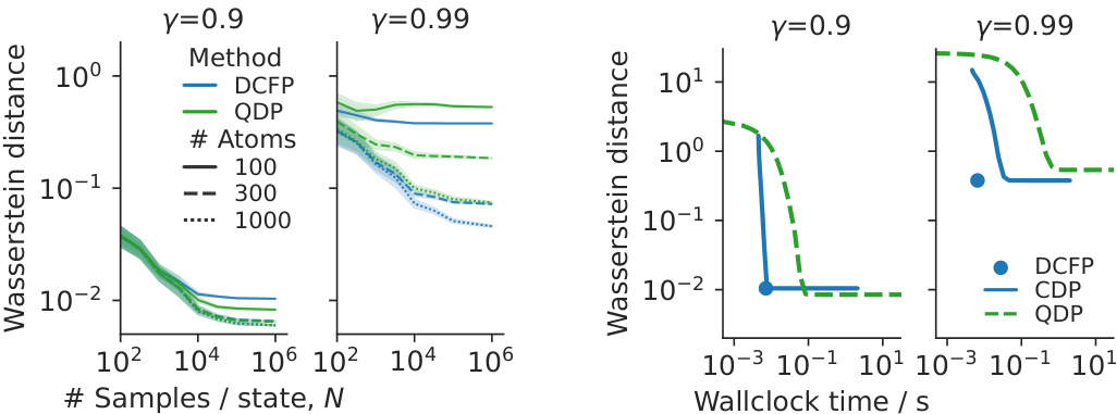
This figure compares the performance of several distributional reinforcement learning methods (DCFP, QDP, CDP) across various settings. It shows the approximation error (Wasserstein distance) and wall-clock time required to achieve this error as a function of the number of samples per state. The results are presented for different discount factors (γ), numbers of atoms (m) used to approximate the distribution, and number of environment samples. The figure helps to understand the trade-offs between accuracy, computational cost, and sample efficiency for each algorithm under different conditions.

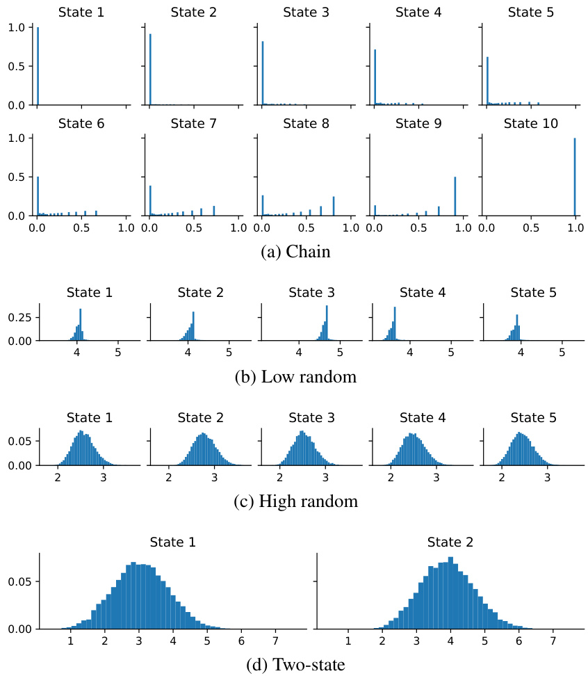
This figure shows the Monte Carlo approximations of the return distributions for the four environments in the paper: Chain, Low random, High random, and Two-state. Each subplot represents a different environment and shows the distribution of returns for each state in that environment. The distributions are estimated using Monte Carlo sampling, and show the variability of returns in each environment.

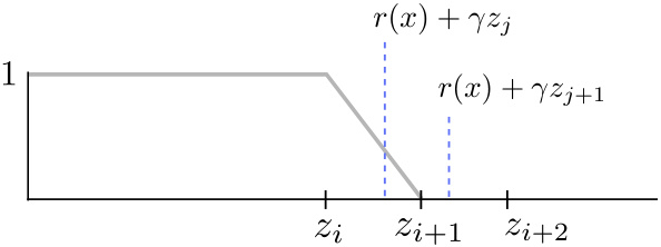
This figure illustrates the categorical dynamic programming approach to distributional reinforcement learning. Panel (a) shows how a continuous distribution is projected onto a discrete set of atoms. Panel (b) shows the effect of the Bellman operator on a categorical distribution and how it is subsequently projected back onto the discrete set of atoms. Finally, Panel (c) shows the hat functions used to perform the projection.

This figure compares the performance of various distributional reinforcement learning algorithms (DCFP, QDP, CDP) across different experimental conditions. The x-axis represents either the number of samples used or the wall-clock time. The y-axis represents the approximation error (Wasserstein distance). The plots show how the algorithms perform under different discount factors (γ), numbers of atoms (m—used in categorical representations), and numbers of environment samples. This allows for analysis of the trade-off between accuracy and computational cost for each algorithm.

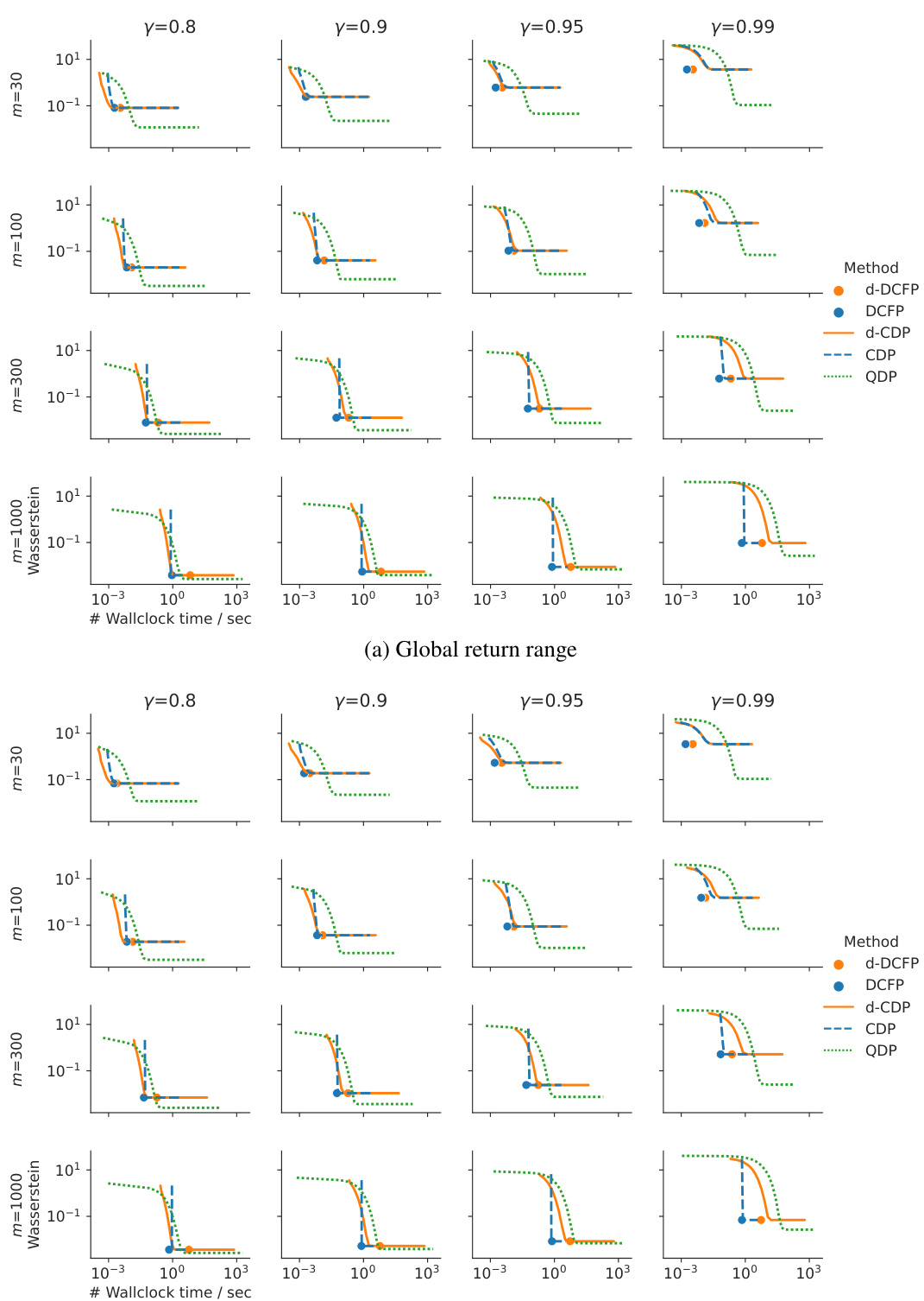
This figure compares the performance of several distributional reinforcement learning algorithms (DCFP, QDP, CDP) in terms of approximation error and computation time. The results are shown for different discount factors (γ), numbers of atoms (m), and numbers of environment samples (N). The figure helps illustrate the trade-off between accuracy and computational cost for different algorithms and parameter settings, offering insights into the practical considerations for choosing an appropriate approach and configuration for specific use cases.

This figure compares the performance of several distributional reinforcement learning algorithms (DCFP, QDP, CDP) under different experimental conditions. The x-axis represents either the number of samples used to estimate the transition probabilities or the wall-clock time, while the y-axis shows the maximum Wasserstein-1 distance between the estimated return distribution and the true distribution (estimated via Monte Carlo). Different lines represent different algorithms and numbers of atoms used for approximation. The results demonstrate that DCFP and QDP show better performance at high discount factors than CDP, with DCFP demonstrating faster execution than QDP. The impact of environmental stochasticity on algorithm performance is also shown.

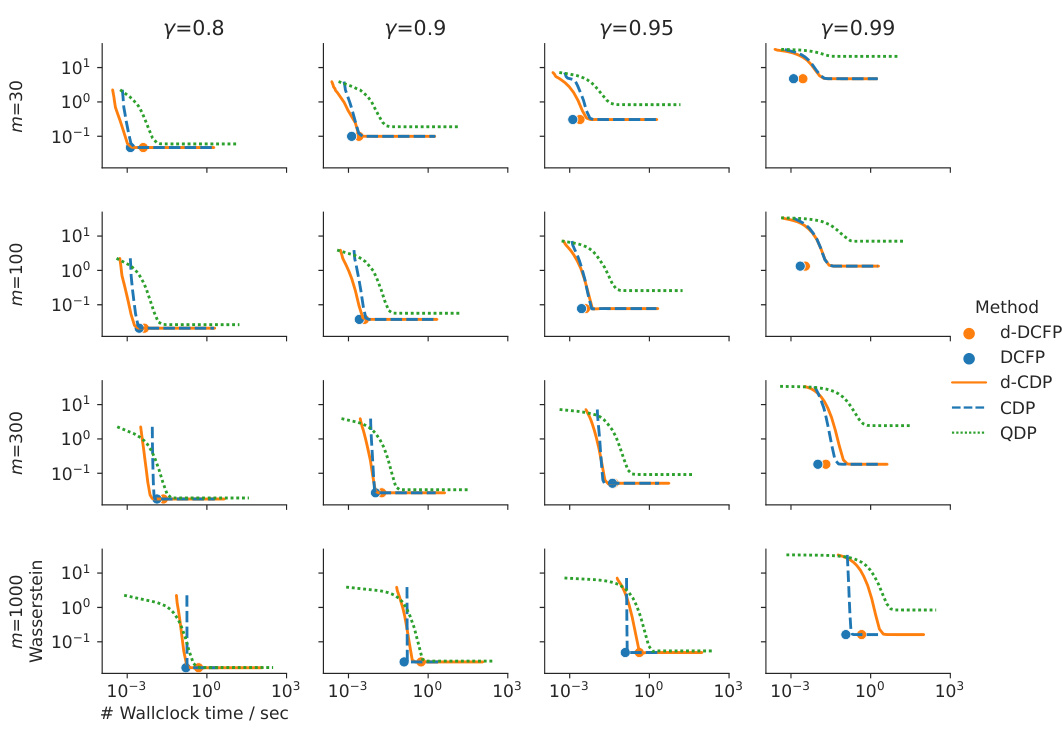
This figure compares the performance of several distributional reinforcement learning algorithms in terms of approximation error and wall-clock time. The algorithms include DCFP, QDP, and CDP, with variations in the number of atoms (representing the granularity of the distribution approximation) used. The experiment varies discount factors and numbers of environment samples to assess performance under different conditions. The results demonstrate a trade-off between accuracy and computational cost. Different algorithms perform better under different conditions, highlighting the importance of algorithm choice based on the specifics of the environment and task.

This figure compares the performance of DCFP and QDP algorithms across various settings, such as different discount factors (γ) and number of atoms (m). It shows how the supremum Wasserstein distance between the estimated return distribution and the true return distribution changes as the number of samples used to estimate the transition matrix (N) increases. The results are presented for four different environments: Chain, Low random, High random, and Two-state, highlighting the impact of environment stochasticity on algorithm performance. The figure also shows results for two atom support settings: using the global return range and using environment-specific return range.

Full paper

#