Rejection via Learning Density Ratios

JzcIKnnOpJ

Alexander Soen et el.

TL;DR
#

Many machine learning applications demand reliable predictions, making rejection crucial when uncertainty is high. Traditional methods modify loss functions, but this paper proposes a distributional approach. It identifies an ‘idealized’ data distribution maximizing model performance and uses a density ratio to compare it with the actual data. This determines rejections, leading to models that are more accurate and robust in uncertain conditions. The method utilizes f-divergences for regularization, extending beyond the typical KL-divergence.

The proposed framework offers a new perspective, unifying existing rejection methods and generalizing well-known rules like Chow’s. It introduces new ways to construct and approximate these idealized distributions, particularly with alpha-divergences. The theoretical results show links to Distributional Robust Optimization and Generalized Variational Inference. Empirical studies on several datasets showcase its effectiveness, especially in handling noisy data, and achieve state-of-the-art results.

Key Takeaways
#

Why does it matter?
#

This paper is important because it offers a novel approach to classification with rejection, a critical problem in machine learning. It provides a theoretical framework grounded in density ratio estimation and idealized distributions, which can lead to improved model robustness and performance in real-world settings where incorrect predictions are costly. The new framework generalizes existing methods, offering a unified perspective and potentially more efficient algorithms. It provides avenues for future work in developing optimal rejection policies and improving the reliability of model predictions in various domains.

Visual Insights
#

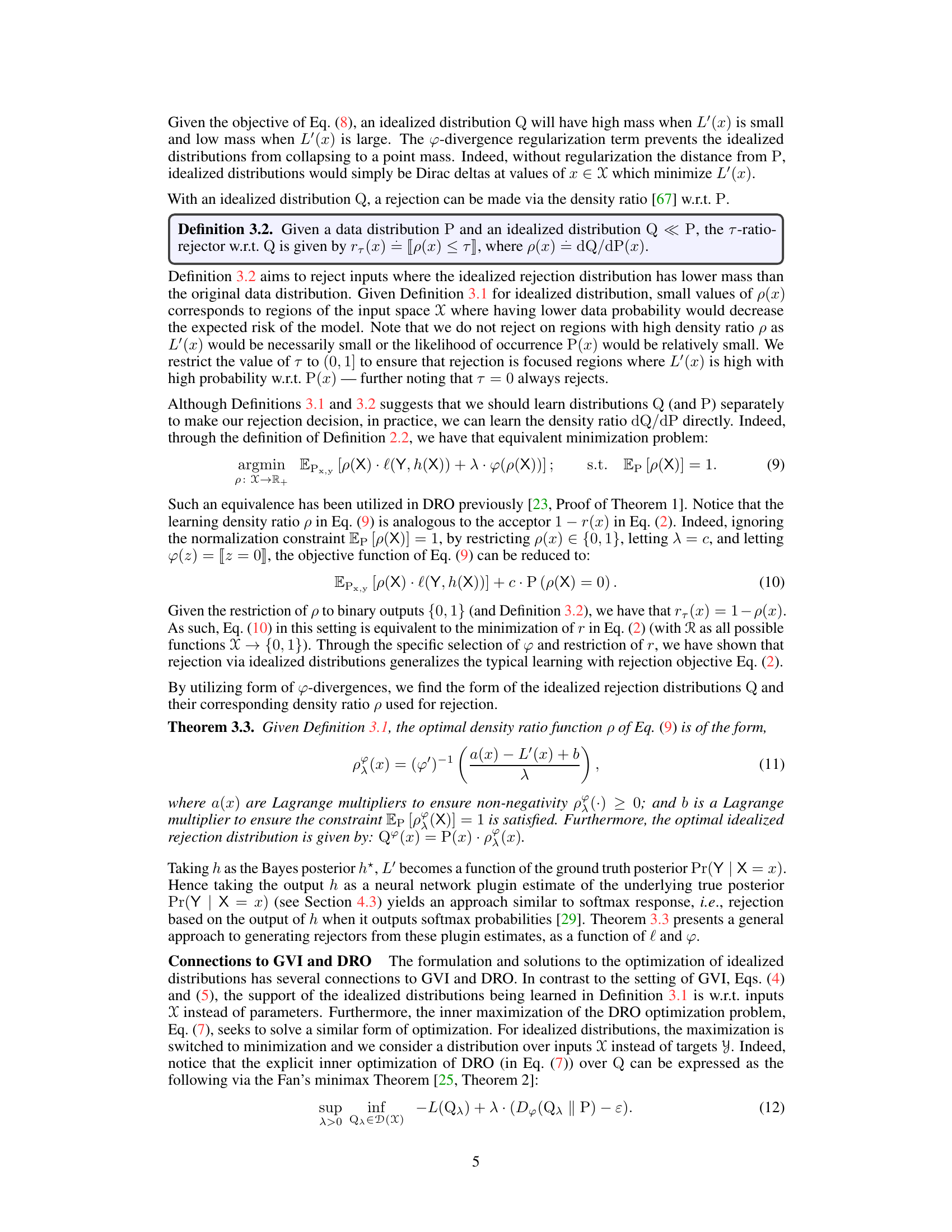
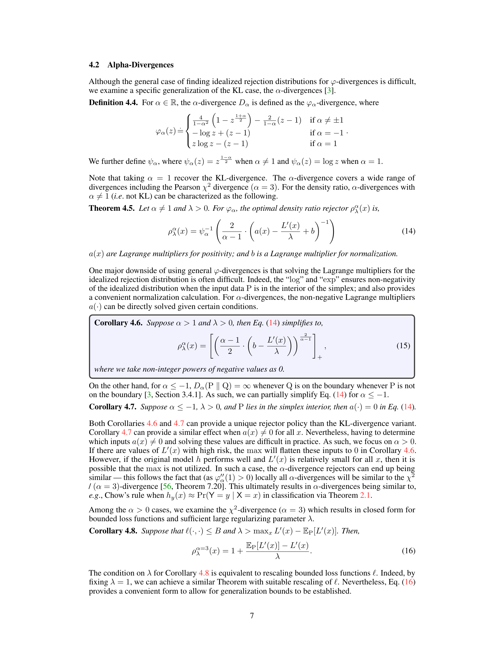
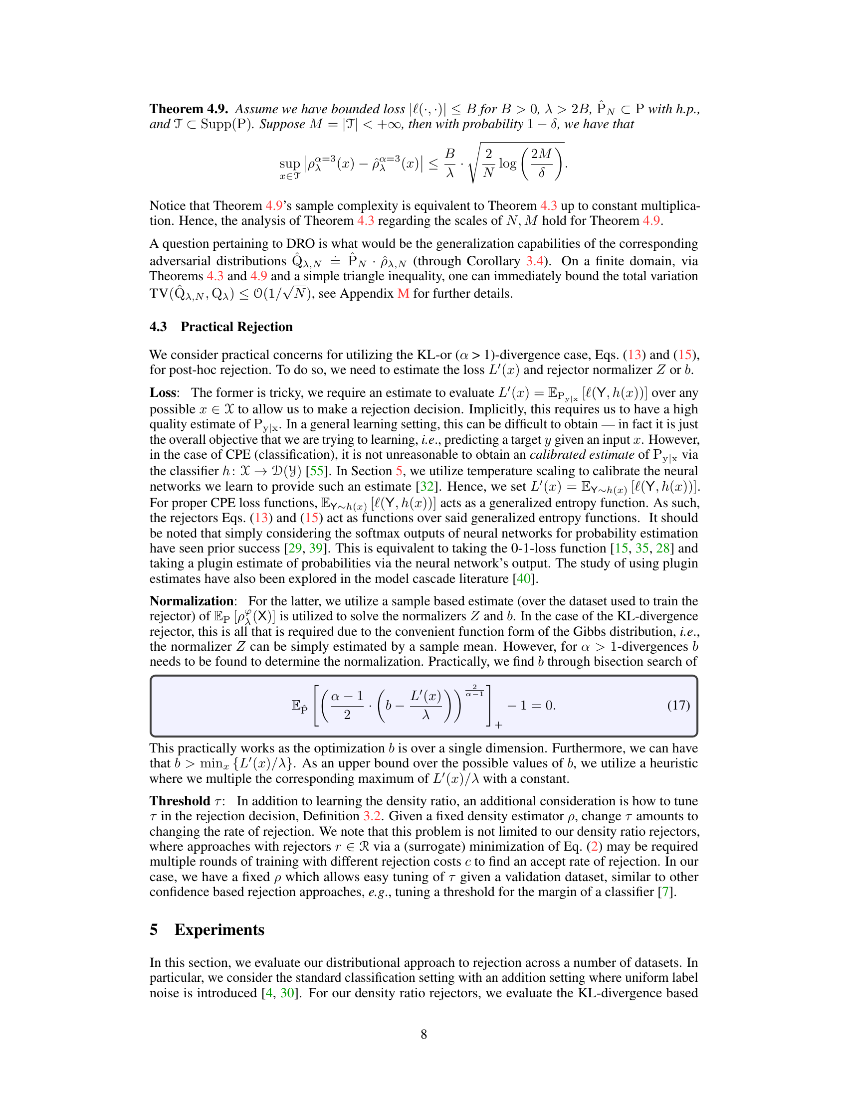
The figure shows two distributions, P (data distribution) and Q (idealized distribution). A density ratio, p(x) = dQ/dP(x), is calculated to compare the two. A rejection criterion is established: if p(x) is below a threshold T, the model abstains from making a prediction. The idealized distribution Q is learned to optimize the model’s performance, so regions where Q has significantly less mass than P represent areas where the model is less confident and thus rejection is preferred.

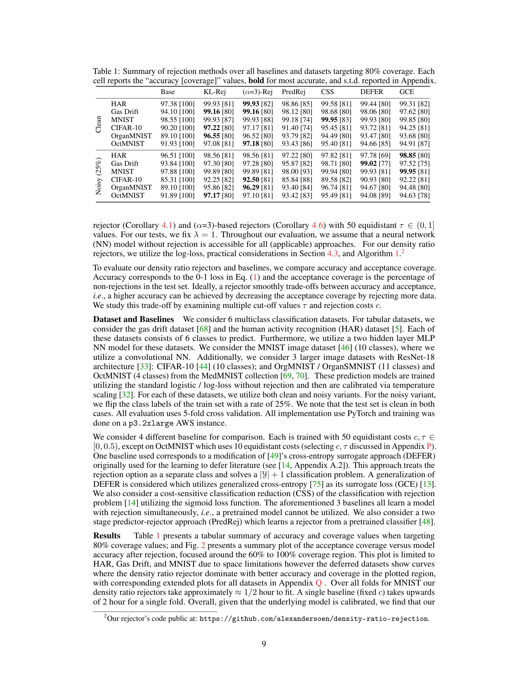
This table summarizes the performance of different rejection methods across various datasets. It compares the accuracy and coverage (percentage of non-rejected instances) achieved by the proposed density-ratio rejection methods against several baseline rejection techniques. The results are shown for both clean and noisy datasets, and the standard deviations are provided in the appendix.

In-depth insights
#

Density Ratio Rej.
#

The proposed ‘Density Ratio Rejection’ method offers a novel approach to selective classification by learning an idealized data distribution that optimizes a pre-trained model’s performance. This approach shifts from traditional loss function modifications to a distributional perspective, using density ratios to compare the idealized distribution with the actual data distribution. A key advantage is the ability to leverage pre-trained models, avoiding the need to train models from scratch. The framework is theoretically grounded, connecting to the established concepts of Distributionally Robust Optimization and Generalized Variational Inference. Empirical evaluations on clean and noisy datasets demonstrate the effectiveness of the proposed method, showing competitiveness or superiority against existing techniques across various datasets and label noise conditions.

Idealized Dist. Learn.
#

The concept of ‘Idealized Dist. Learn.’ in a machine learning context likely refers to a method for learning an optimal data distribution that maximizes a model’s performance. This approach contrasts with traditional methods that directly optimize model parameters. Instead of focusing on the model itself, it focuses on the data the model operates on. A key idea is to identify an idealized distribution – a theoretical data distribution where the model would achieve its best performance. By comparing this idealized distribution to the real data, one can make informed decisions about how to improve the model’s accuracy, including potentially rejecting uncertain predictions. This method offers a different perspective on model improvement, shifting the focus from modifying the model to improving the data input. Successful implementation of this technique would depend heavily on how well the idealized distribution is defined and approximated, as well as the method used to compare it to real-world data. The effectiveness also hinges on the model’s ability to generalize beyond the idealized distribution. Further exploration into this technique could provide novel insights into robust machine learning and selective classification.

GVI & DRO Links
#

The conceptual link between Generalized Variational Inference (GVI) and Distributionally Robust Optimization (DRO) offers a powerful lens for analyzing rejection mechanisms in machine learning. GVI’s focus on finding an idealized data distribution that optimizes model performance directly parallels DRO’s goal of minimizing risk under worst-case distributional uncertainty. This shared distributional perspective is key. By framing rejection as a comparison between the learned idealized distribution and the actual data distribution, we gain a unified theoretical framework encompassing both GVI and DRO. The density ratio between these distributions becomes a natural rejector, providing a principled way to abstain from predictions where model confidence is low relative to the idealized scenario. This framework elegantly connects existing rejection approaches with broader distributional robustness concepts, offering valuable insights into the theoretical underpinnings of rejection learning. Consequently, it opens up new avenues for developing more robust and reliable rejection techniques.

Practical Rej. App.
#

The section “Practical Rejection Applications” would delve into the real-world implementation challenges and solutions for the proposed rejection methods. It would likely discuss practical considerations for estimating the loss function and density ratio, emphasizing the importance of calibrated probability estimates for effective rejection. Approaches for handling the computational cost of calculating density ratios for large datasets would be explored, potentially including approximation techniques or sampling methods. The section would also address the critical issue of threshold selection for the rejector, explaining how to effectively determine the optimal threshold to balance accuracy and rejection rate. A key aspect would be the evaluation of the practical rejection framework on real-world datasets, highlighting its performance in various scenarios and comparing it with existing rejection methods. Finally, the discussion would likely touch upon the limitations of the approach in practical settings and potential future research directions for improvement.

Future Work
#

Future research directions stemming from this work on rejection via learning density ratios could explore several promising avenues. Improving the efficiency and scalability of the proposed algorithms, especially for high-dimensional input spaces, is crucial for practical applications. Investigating alternative divergence functions beyond the α-divergences, such as integral probability metrics, could lead to more robust and flexible rejection methods. Addressing the limitation of relying on an existing pre-trained model for generating the density ratios is key. Exploring methods to directly learn both the idealized and data distributions simultaneously, or to learn the density ratio without relying on a pre-trained classifier, could enhance performance and reduce the reliance on assumptions about the pre-trained model’s calibration. Finally, extending the framework to handle more complex scenarios such as handling noisy labels, imbalanced datasets, or settings with concept drift would greatly broaden the applicability of this promising technique.

More visual insights
#

More on figures

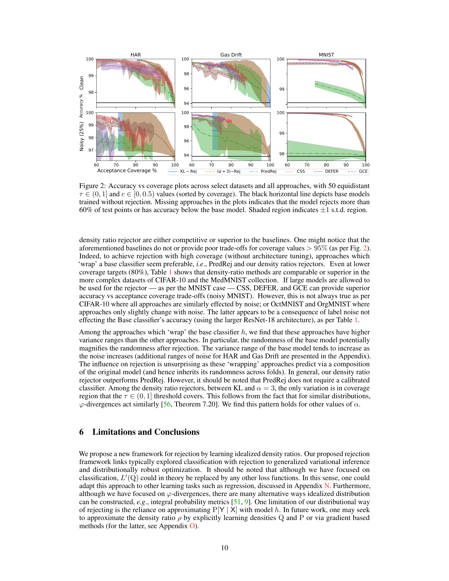
This figure compares the performance of different rejection methods across three datasets (HAR, Gas Drift, MNIST) at various acceptance coverage levels. Each method’s accuracy is plotted against its acceptance coverage, with the black horizontal line representing the baseline accuracy without rejection. The shaded areas represent the standard deviation. Missing points indicate that the model rejected more than 60% of test points or achieved an accuracy below the baseline.

This figure compares the performance of different rejection methods across multiple datasets, showing the trade-off between accuracy and acceptance coverage. Each point represents a specific rejection threshold. The black line shows the baseline accuracy without rejection. The shaded area represents the standard deviation, indicating variability. Missing data points signify that the model rejected more than 60% of the data or performed worse than the baseline.

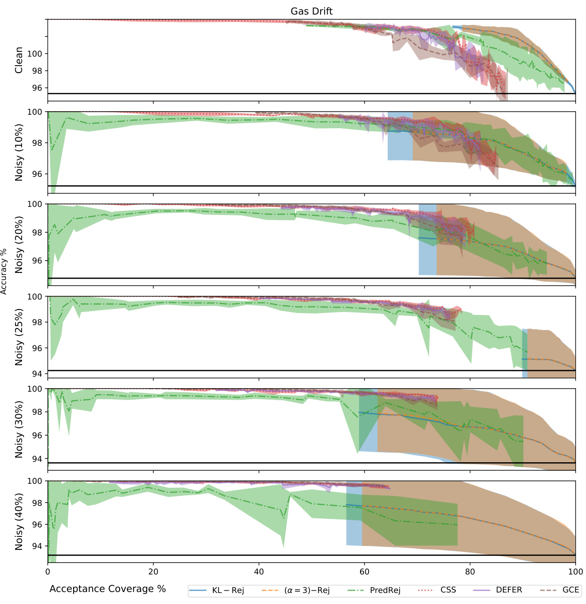
The figure shows the accuracy vs. acceptance coverage trade-off for different rejection methods on three datasets (HAR, Gas Drift, MNIST). Each method is represented by a line showing its performance across different thresholds (τ). The black horizontal line represents the baseline accuracy without rejection. The shaded area indicates the standard deviation. Missing data points indicate that a particular method rejected more than 60% of the data points or had lower accuracy than the baseline model. This figure illustrates the performance of the proposed density ratio rejection method compared to alternative approaches.

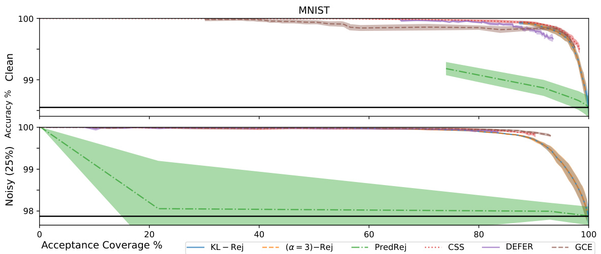
This figure compares the performance of different rejection methods, including the proposed density ratio rejection methods, on three datasets (HAR, Gas Drift, MNIST) under clean and noisy conditions. The x-axis represents the acceptance coverage (percentage of inputs not rejected), while the y-axis shows the accuracy. The plots illustrate how each method trades off accuracy for coverage. The black horizontal line represents the baseline performance without rejection. Shaded areas represent one standard deviation around the mean.

The figure shows the accuracy vs. acceptance coverage trade-off for different rejection methods on three datasets (HAR, Gas Drift, and MNIST). Each method is represented by a line, showing how the model’s accuracy changes as the acceptance coverage (percentage of instances not rejected) varies. The black horizontal line indicates the accuracy of the base model without any rejection. The shaded area shows the standard deviation around the mean accuracy for each point.

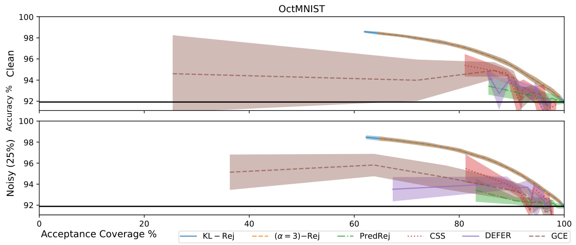
This figure shows the accuracy vs. acceptance coverage trade-off for various rejection methods on several datasets. Each point represents a different threshold for rejection. The black horizontal line indicates the baseline accuracy without rejection. Shaded areas represent standard deviations.

This figure compares the performance of various rejection methods, including the proposed density ratio rejectors, against baselines on three datasets (HAR, Gas Drift, MNIST). Each method’s accuracy is plotted against its acceptance coverage (percentage of instances not rejected), for different threshold values (τ). The black horizontal line shows the accuracy of the base model without rejection. The shaded region represents the standard deviation. Methods that frequently reject (rejecting > 60% of instances) or perform worse than the base model are omitted from the plots.

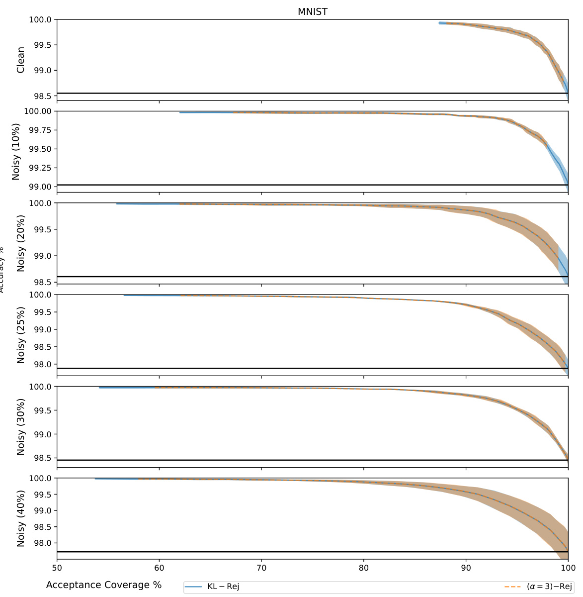
The figure shows the accuracy versus acceptance coverage plots for MNIST dataset with different levels of label noise (10%, 20%, 25%, 30%, 40%). The plots compare the performance of two density ratio rejection methods: KL-Rej and (α=3)-Rej. Each line represents a specific noise level, and the shaded area represents the standard deviation. The figure illustrates how the rejection methods trade-off accuracy and coverage under varying levels of data corruption.

This figure compares the accuracy and coverage of different rejection methods, including the proposed density ratio methods and several baselines. The x-axis represents the acceptance coverage (percentage of inputs not rejected), and the y-axis represents the accuracy. Each point represents a different threshold value, and the lines connect points with similar thresholds. The black horizontal lines show the baseline accuracy without rejection. The shaded region represents the standard deviation of the accuracy. The plot shows that the density-ratio rejectors generally provide a better tradeoff between accuracy and coverage than the baselines, particularly when a higher coverage is required. Some methods are missing from certain plots because their rejection rates are too high.

This figure displays the accuracy vs. acceptance coverage trade-off for different rejection methods on three datasets: HAR, Gas Drift, and MNIST. The x-axis represents acceptance coverage (percentage of inputs not rejected), and the y-axis shows the accuracy of the model on the accepted inputs. Each method is represented by a line, with the shaded area representing one standard deviation. The black horizontal line indicates the baseline accuracy without rejection. The plot demonstrates how different methods balance accuracy and rejection rate.

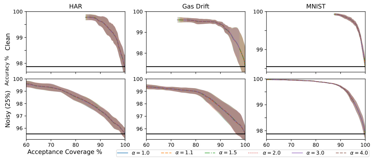
This figure displays the accuracy versus acceptance coverage trade-off for different rejection methods on three datasets (HAR, Gas Drift, MNIST). Each point represents a model trained with a different rejection threshold, and the lines connect points with the same method. The black horizontal line shows the baseline accuracy without rejection. The shaded area represents the standard deviation of the results. The plot shows that the density-ratio rejection method (KL-Rej and α=3-Rej) achieves high accuracy even at high coverage rates, outperforming other methods in many cases.

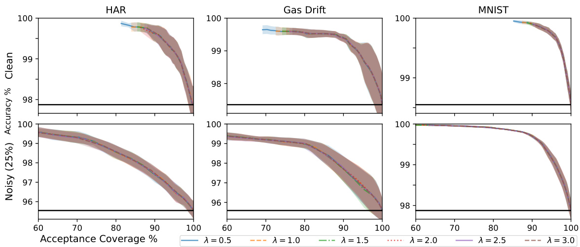
This figure shows the accuracy vs. acceptance coverage trade-off for different rejection methods on three datasets: HAR, Gas Drift, and MNIST. Each point represents a different threshold (τ) used for rejection. The black line represents the baseline model without rejection. The shaded area represents the standard deviation. The plot illustrates how each method balances accuracy and rejection rate, allowing a model to reject predictions it’s less confident about in order to improve overall accuracy.