↗ OpenReview ↗ NeurIPS Homepage ↗ Chat
TL;DR#
Deep Neural Networks (DNNs) are powerful but lack the clear statistical interpretation and precise semantics of Probabilistic Graphical Models (PGMs). This creates challenges in understanding and improving DNNs. Existing attempts to bridge this gap are limited.
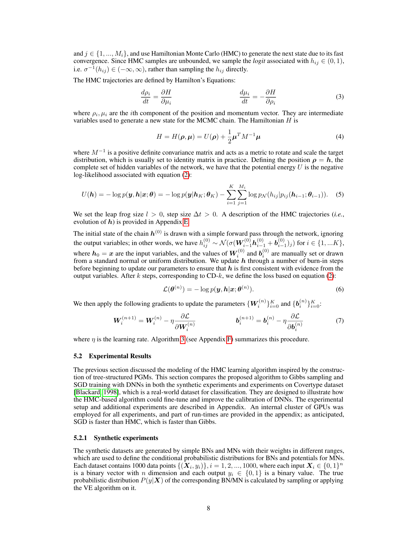
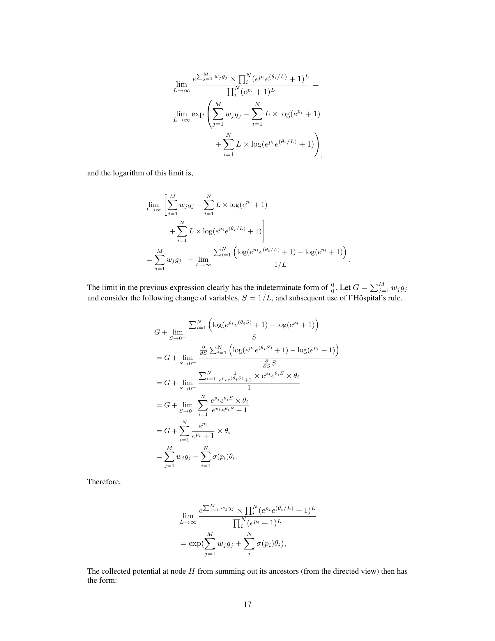
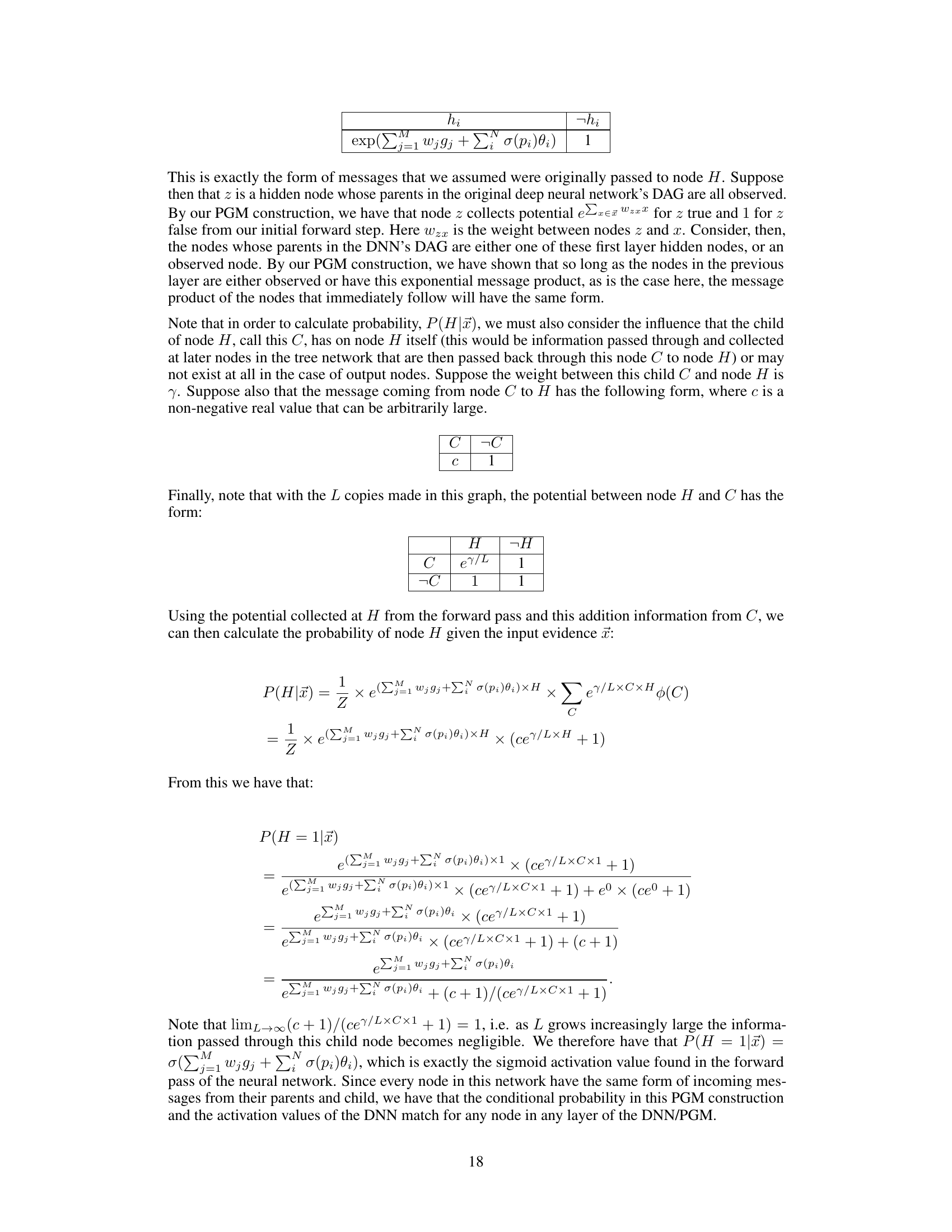
This paper proposes a novel approach by constructing infinite tree-structured PGMs that perfectly match DNNs. It proves that the forward pass of a DNN is essentially performing an approximate inference in this equivalent PGM structure. This discovery has significant implications for better understanding and interpreting DNNs. The method also suggests opportunities for developing new algorithms by combining the advantages of both PGMs and DNNs, paving the way for more powerful and explainable AI systems. Empirical results demonstrate the effectiveness of using Hamiltonian Monte Carlo sampling within this framework for improved model calibration.
Key Takeaways#
Why does it matter?#
This paper is crucial for AI researchers seeking to bridge the gap between the interpretability of probabilistic graphical models (PGMs) and the high performance of deep neural networks (DNNs). It offers new algorithms for training and interpreting DNNs, providing improved calibration and clear statistical semantics. The proposed approach opens exciting avenues for future research by integrating the strengths of both PGMs and DNNs in developing more explainable and robust AI systems.
Visual Insights#
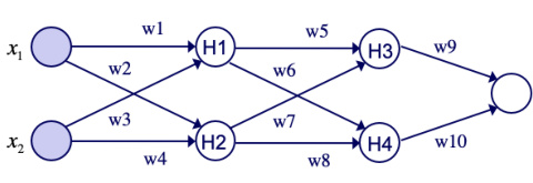
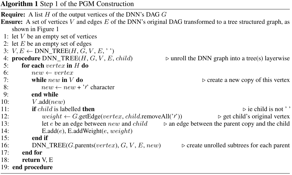
This figure illustrates the first step in constructing a tree-structured probabilistic graphical model (PGM) that corresponds to a given deep neural network (DNN). The original DNN is shown in (a), illustrating its structure with shared latent variables (H1 and H2). In (b), the first step of the PGM construction is shown, where these shared latent parents are separated into copies. Each copy is only connected to one child of the original latent variable, replicating the entire ancestral subtree for each copy. This process continues for each layer of the network until separate trees are formed for each output node.
This table presents the results of calibration performance experiments on synthetic datasets using different training methods (DNN, Gibbs sampling, and HMC with varying L values). The mean absolute error (MAE) is reported for each method, along with p-values from t-tests comparing the MAE of Gibbs and HMC to SGD. Highlighted cells indicate statistically significant improvements in MAE for Gibbs and/or HMC over SGD.
In-depth insights#
DNN-PGM Bridge#
The concept of a ‘DNN-PGM Bridge’ signifies a crucial effort to unify deep neural networks (DNNs) and probabilistic graphical models (PGMs). Bridging this gap is essential because DNNs excel at complex pattern recognition but lack interpretability, while PGMs offer clear probabilistic semantics but often struggle with the scale and complexity of real-world data. A successful bridge would ideally leverage the strengths of both, yielding models that are both powerful and interpretable. This might involve representing DNNs as specific types of PGMs, potentially infinite tree-structured ones, allowing for the application of PGM inference techniques to DNNs. Alternatively, it could involve developing algorithms that seamlessly integrate PGM reasoning within the DNN training process. The key challenge lies in finding a mapping that accurately captures the complexities of DNN behavior within the framework of PGMs. Success would lead to improved model interpretability, calibration, and the ability to incorporate existing PGM methods for tasks like uncertainty quantification. This research direction promises to greatly improve our understanding and application of deep learning.
Infinite-Tree PGMs#
The concept of “Infinite-Tree PGMs” offers a novel perspective on deep neural networks (DNNs). It proposes representing DNNs as infinite-width tree-structured probabilistic graphical models (PGMs). This framework provides a precise probabilistic interpretation for DNNs, moving beyond the limitations of purely functional interpretations. The core idea is that forward propagation in a DNN corresponds exactly to approximate inference within this infinite PGM. This elegant correspondence enables a deeper understanding of DNN behavior, offering improved pedagogy and interpretability. Furthermore, it suggests the possibility of integrating PGM algorithms with DNNs, leveraging the strengths of both approaches for tasks like improved calibration or Bayesian inference. While theoretically elegant, the infinite nature of the model poses practical challenges, demanding further exploration of approximation techniques and efficient algorithms.
HMC for DNNs#
The application of Hamiltonian Monte Carlo (HMC) to deep neural networks (DNNs) offers a compelling approach to address limitations in traditional DNN training. HMC’s probabilistic framework aligns well with the inherent uncertainty in DNNs, leading to better calibrated predictions and improved uncertainty quantification. By treating DNNs as infinite tree-structured probabilistic graphical models, the authors elegantly connect the forward pass of a DNN with exact inference in a corresponding PGM. This theoretical framework justifies the use of HMC, which addresses the shortcomings of standard gradient-based methods. Fine-tuning a DNN with HMC, after initial SGD training, empirically demonstrates improved calibration, showing potential for enhancing the reliability and interpretability of DNNs. The theoretical foundation and empirical evidence suggest that HMC can be a powerful tool for refining DNNs, potentially leading to more robust and trustworthy AI systems.
Calibration & Limits#
Calibration is crucial for reliable probabilistic predictions from deep neural networks (DNNs). This paper investigates how DNNs, interpreted as infinite tree-structured probabilistic graphical models (PGMs), impact calibration. The infinite width of the PGM allows the derivation of precise semantics and definitive probabilistic interpretations of DNN forward propagation. However, the infinite nature poses challenges for practical application. The research demonstrates that DNN training, particularly with standard gradient methods, does not exactly align with the PGM semantics. While the correspondence of the forward pass is exact for sigmoid activations, the incompatibility with the training gradient raises calibration issues. The proposed solutions address the challenge using advanced Markov Chain Monte Carlo (MCMC) methods that efficiently improve calibration by approximating the Gibbs sampling process. This study, therefore, highlights a trade-off between theoretical elegance and practical limitations, emphasizing the need for exploring algorithm modifications to reconcile these aspects.
Future Directions#
The research paper explores the exciting intersection of deep neural networks (DNNs) and probabilistic graphical models (PGMs). Future directions could involve extending the theoretical framework to encompass a broader range of activation functions beyond sigmoid, and rigorously analyzing the approximations inherent in using layer normalization or batch normalization as proxies for proper normalization. Investigating the practical implications of using PGMs algorithms like contrastive divergence or Hamiltonian Monte Carlo to enhance DNN training, calibration and interpretation would be highly valuable. Exploring alternative methods for approximating inference in larger, non-tree-structured PGMs would be a significant advance. Finally, the potential of applying these insights to real-world problems in areas like genomics and gene regulatory networks should be a focal point of further research, ensuring a practical impact alongside theoretical advancement.
More visual insights#
More on tables
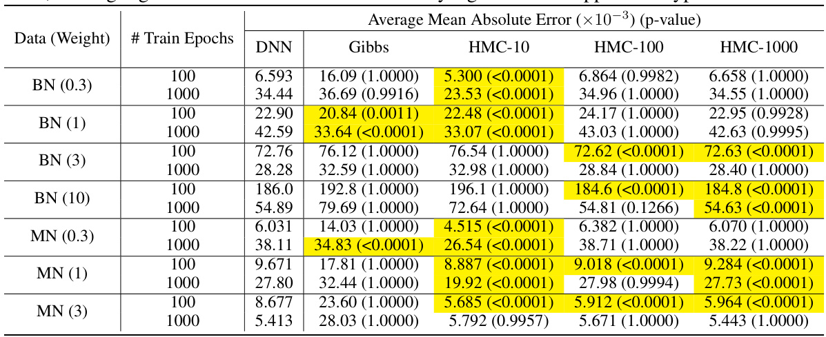
This table presents the results of calibration experiments on synthetic datasets generated using Bayesian networks (BNs) and Markov networks (MNs) with varying weight parameters. The table compares the mean absolute error (MAE) of predictions from a deep neural network (DNN) trained using stochastic gradient descent (SGD), fine-tuned with Gibbs sampling and Hamiltonian Monte Carlo (HMC) methods. The p-values from t-tests comparing the MAE of Gibbs sampling and HMC methods to SGD are also reported, highlighting statistically significant improvements in calibration accuracy for some methods.

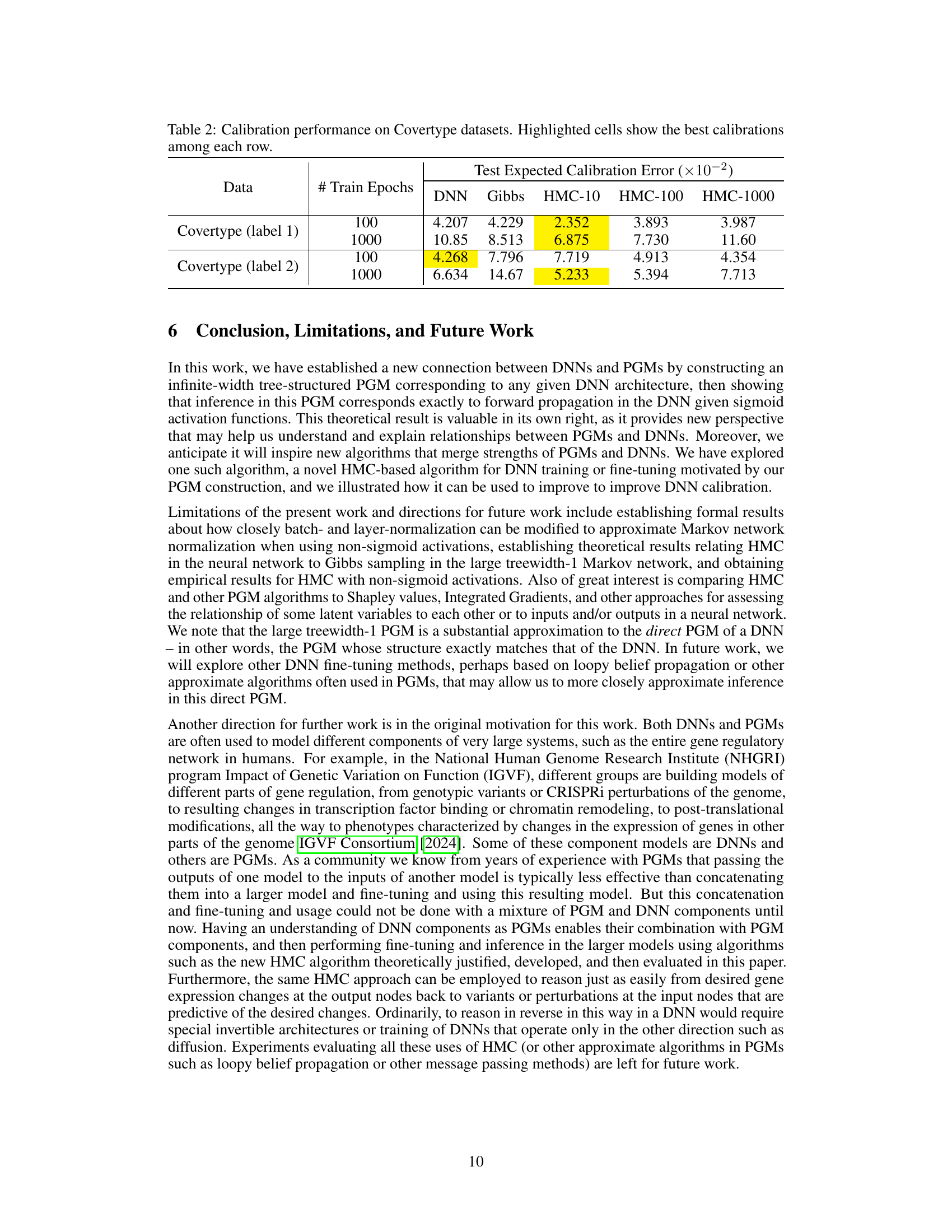
This table presents the results of calibration experiments on the Covertype dataset. It compares the performance of three methods: SGD (DNN), Gibbs sampling, and the proposed Hamiltonian Monte Carlo (HMC) algorithm. The table shows the test expected calibration error (ECE) for different training epochs (100 and 1000) and different HMC parameters (L=10, L=100, L=1000). Highlighted cells indicate the lowest ECE for each row (dataset/training epoch combination). The results demonstrate the impact of the proposed HMC algorithm for improving model calibration.
This table presents the mean absolute error (MAE) in model calibration for different training methods (DNN, Gibbs sampling, and Hamiltonian Monte Carlo with different numbers of copies) on synthetic datasets (Bayesian networks and Markov networks with varying weights). The table shows MAE values and p-values from t-tests comparing the different training methods. Highlighted cells indicate statistically significant improvements in MAE compared to standard DNN training.

This table presents the results of calibration experiments using synthetic datasets generated from Bayesian Networks (BNs) and Markov Networks (MNs). The experiments compare the performance of three methods: DNN (deep neural network) training with SGD (stochastic gradient descent), Gibbs sampling, and HMC (Hamiltonian Monte Carlo) with different values of hyperparameter L. The table shows the mean absolute error (MAE) for each method on various datasets with different weight settings. Highlighted p-values indicate statistical significance when comparing Gibbs and HMC to SGD.

This table presents the mean absolute error (MAE) in model calibration for different training methods (DNN, Gibbs, and HMC with various L values) across several synthetic datasets. Each dataset is trained for 100 or 1000 epochs using SGD and then fine-tuned with Gibbs or HMC for 20 epochs. The MAE is calculated by comparing the predicted probabilities from the fine-tuned networks with the true probabilities. Statistical significance is assessed via t-tests. Highlighted cells show statistically significant improvements over SGD.

This table presents the mean absolute error (MAE) in model calibration for different training methods (DNN, Gibbs sampling, and HMC with different L values) on synthetic datasets. The MAE measures the difference between predicted probabilities and true probabilities. The results are based on 100 runs per experiment for each model. Statistical significance tests (t-tests) are performed to compare different training methods, highlighting when the difference is statistically significant.

The table presents the results of calibration experiments on synthetic datasets using three methods: DNN, Gibbs sampling, and Hamiltonian Monte Carlo (HMC). For each method and dataset, the mean absolute error (MAE) is reported, along with p-values from t-tests comparing the MAE of Gibbs and HMC to SGD. Highlighted values indicate statistically significant differences (p<0.05). The experiments are designed to assess the impact of fine-tuning a pre-trained DNN using Gibbs sampling and HMC on model calibration performance, particularly with variations in network weights (0.3, 1, 3, 10). The results demonstrate that fine-tuning with HMC can improve model calibration.

This table presents the mean absolute error (MAE) results for different models (DNN, Gibbs sampling, and HMC with different L values) on synthetic datasets. The results are averaged over 100 runs to reduce the impact of randomness. Statistical significance tests (t-tests) are performed to determine if Gibbs sampling and HMC yield lower MAE values than standard SGD training. Highlighted cells in the table indicate statistically significant improvements (p<0.05). The table shows results for both Bayesian Networks (BNs) and Markov Networks (MNs) with varying weight scales to examine the influence of weight magnitude on model calibration.

This table presents the results of calibration experiments on synthetic datasets generated by Bayesian Networks (BNs) and Markov Networks (MNs). Different network weights and training epochs are used, and performance is measured by Mean Absolute Error (MAE). The table compares the MAE of models trained with Stochastic Gradient Descent (SGD), Gibbs sampling, and Hamiltonian Monte Carlo (HMC). Highlighted cells indicate statistically significant improvement of Gibbs or HMC compared to SGD. The number of copies (L) used in the HMC method is also varied.

This table presents the results of calibration experiments on synthetic datasets using three different methods: DNN, Gibbs, and HMC with various values of L. The table compares the mean absolute error (MAE) of each method in predicting probabilities, and highlights statistically significant results showing when Gibbs or HMC outperforms SGD. The results demonstrate that HMC, particularly with L=10, generally performs better in terms of calibration, especially for networks with smaller weights.

This table presents the mean absolute error (MAE) results for different models (DNN, Gibbs sampling, and HMC with varying L values) on synthetic datasets (BNs and MNs with varying weights). The MAE is a measure of the model’s calibration, indicating how well the predicted probabilities match the true probabilities. The table compares the performance of the models after training for 100 and 1000 epochs, with additional fine-tuning using Gibbs or HMC for 20 epochs. The statistical significance of the results, comparing Gibbs and HMC to SGD, is indicated using p-values; highlighted cells represent statistically significant improvements.
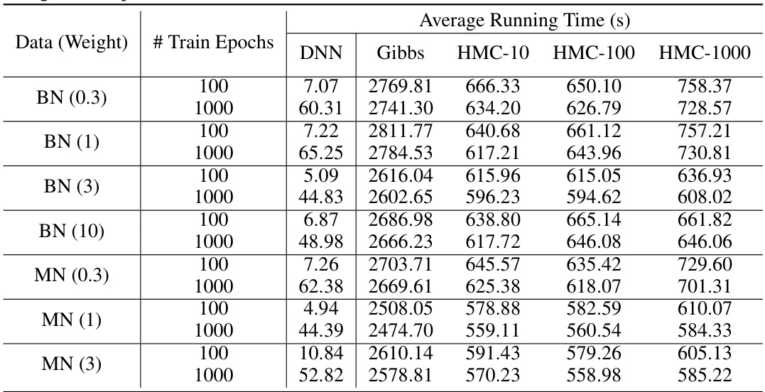
This table presents the results of calibration experiments on synthetic datasets generated from Bayesian Networks (BNs) and Markov Networks (MNs). It compares the Mean Absolute Error (MAE) of three different fine-tuning methods (Gibbs sampling, Hamiltonian Monte Carlo with L=10, L=100, and L=1000) against the performance of a Deep Neural Network (DNN) trained with Stochastic Gradient Descent (SGD). The table shows the MAE for each method, along with p-values from t-tests comparing the fine-tuning methods to SGD. Highlighted p-values indicate statistically significant improvements in MAE.
Full paper#


