TL;DR#
Many machine learning tasks involve optimizing complex models using stochastic gradient descent. However, traditional accelerated methods, like Nesterov’s Accelerated Gradient Descent (NAG), struggle when gradient estimates are highly noisy. This noise often arises in overparametrized models, where the number of parameters exceeds the amount of data. The high noise can lead to instability and prevent these methods from reaching their optimal convergence rate.
This paper introduces AGNES (Accelerated Gradient descent with Noisy EStimators), a new algorithm designed to overcome the limitations of NAG in noisy settings. AGNES achieves accelerated convergence regardless of the signal-to-noise ratio, outperforming existing methods, particularly in scenarios with high noise. The algorithm’s parameters have clear geometric interpretations, aiding in practical implementation and parameter tuning for machine learning tasks.
Key Takeaways#
Why does it matter?#
This paper is crucial for researchers in optimization and machine learning because it addresses the limitations of existing accelerated gradient methods in handling noisy gradients, a common challenge in modern machine learning. It provides theoretically sound and practically useful solutions with clear geometric interpretations and heuristics for parameter tuning, opening new avenues for research and improving the efficiency of training complex models.
Visual Insights#

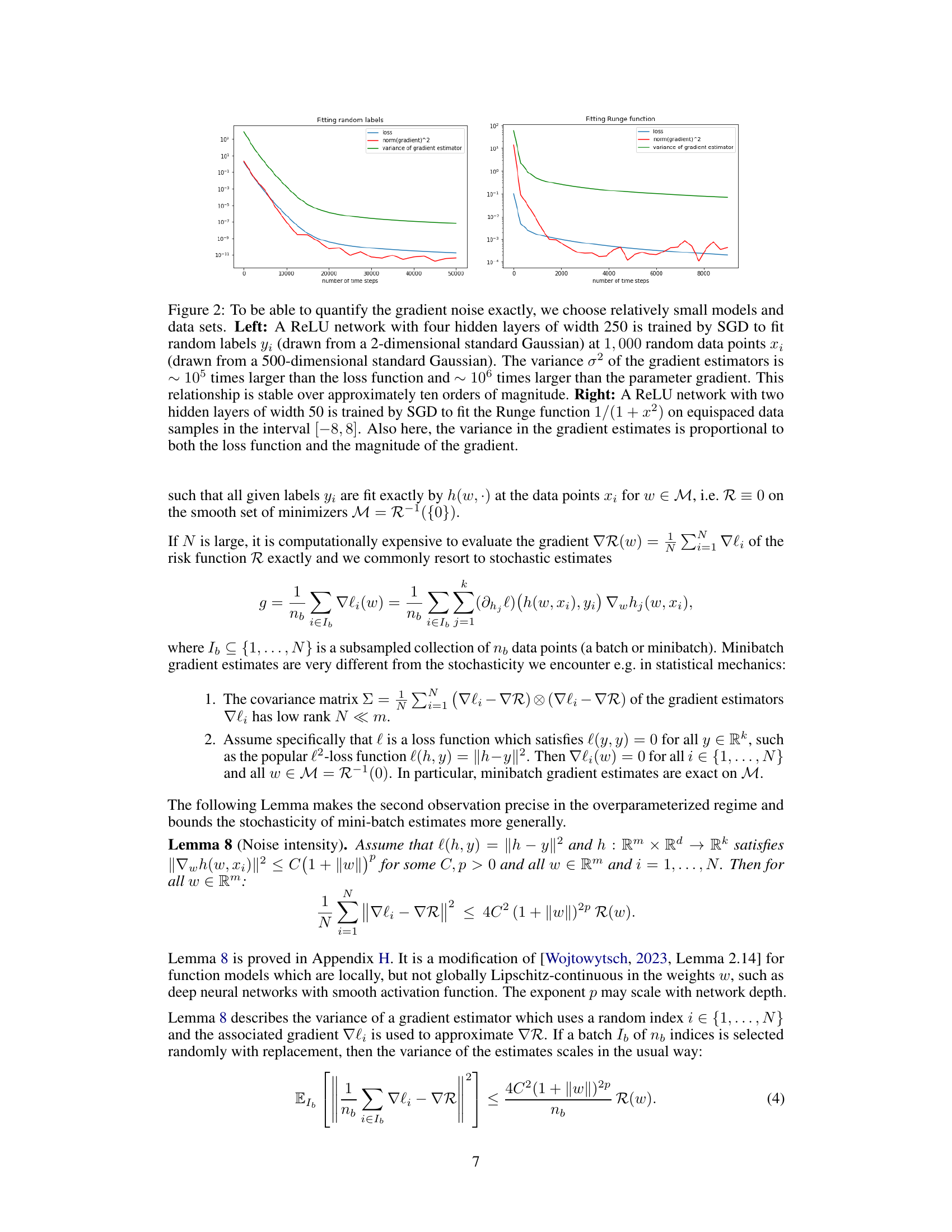
🔼 The figure shows empirical evidence supporting the multiplicative noise assumption. Two experiments are presented: one fitting random labels to random data points using a larger network, and one fitting the Runge function to equispaced data points using a smaller network. In both cases, the variance of the gradient estimator scales linearly with both the loss function and the magnitude of the gradient. This supports the paper’s assumption that the noise intensity in the gradient estimates is proportional to the magnitude of the gradient.
read the caption
Figure 2: To be able to quantify the gradient noise exactly, we choose relatively small models and data sets. Left: A ReLU network with four hidden layers of width 250 is trained by SGD to fit random labels yi (drawn from a 2-dimensional standard Gaussian) at 1,000 random data points Xi (drawn from a 500-dimensional standard Gaussian). The variance σ² of the gradient estimators is ~ 105 times larger than the loss function and ~ 106 times larger than the parameter gradient. This relationship is stable over approximately ten orders of magnitude. Right: A ReLU network with two hidden layers of width 50 is trained by SGD to fit the Runge function 1/(1 + x2) on equispaced data samples in the interval [-8, 8]. Also here, the variance in the gradient estimates is proportional to both the loss function and the magnitude of the gradient.

🔼 This table compares the time complexity of the AGNES and SGD algorithms for achieving a target error (ε) in convex and μ-strongly convex optimization problems. It highlights that AGNES requires three hyperparameters (compared to one for SGD) to reach the optimal convergence rate. The table shows the time complexities are dependent on the condition number (L/μ in strongly convex case) and noise intensity (σ).
read the caption
Figure 1: The minimal n for AGNES and SGD such that E[f(xn) - inf f] < ɛ when minimizing an L-smooth function with multiplicative noise intensity σ in the gradient estimates and under a convexity assumption. The SGD rate of the µ-strongly convex case is achieved more generally under a PL condition with PL-constant μ. While SGD requires the optimal choice of one variable to achieve the optimal rate, AGNES requires three (two in the determinstic case).
In-depth insights#
Noisy Gradient#
The concept of a noisy gradient is central to the study of optimization algorithms in contexts where gradients cannot be computed exactly, such as in stochastic gradient descent (SGD) applied to machine learning. Noise arises from approximations used to estimate gradients, often due to the use of mini-batches of data. The paper investigates the impact of noise on the convergence rate and identifies a particular type of noise—multiplicative noise—where the noise intensity is directly proportional to the magnitude of the gradient. This noise model is particularly relevant in overparameterized machine learning scenarios, where exact interpolation is possible, and thus noisy gradients are a consequence of using a subset of the data in each step. The paper introduces a generalized algorithm called AGNES (Accelerated Gradient Descent with Noisy Estimators), which is designed to accommodate this kind of noise and still achieve acceleration. The study highlights the importance of carefully managing noise in optimization, particularly when leveraging gradient-based accelerated methods.
AGNES Algorithm#
The AGNES (Accelerated Gradient descent with Noisy EStimators) algorithm is a novel method designed to address the challenges of accelerating gradient descent in the presence of noisy gradient estimates, particularly in overparameterized machine learning models. AGNES generalizes Nesterov’s accelerated gradient descent method, handling noise intensity proportional to the gradient’s magnitude. Unlike standard Nesterov’s method which only guarantees acceleration under specific signal-to-noise conditions, AGNES provably achieves acceleration regardless of the signal-to-noise ratio. This robustness is achieved through a clever reparameterization of the momentum term. The algorithm’s parameters are interpretable geometrically, providing insights into their optimal choice. AGNES shows improved performance over SGD with momentum and Nesterov’s method in numerical experiments, showcasing its effectiveness in training CNNs and addressing limitations encountered by prior work in handling noisy gradient settings.
Convergence Analysis#
A rigorous convergence analysis is crucial for evaluating the effectiveness and reliability of any optimization algorithm. In this context, a comprehensive analysis would delve into the algorithm’s convergence rates under various conditions, such as convexity, strong convexity, and non-convexity of the objective function. Convergence rates, typically expressed as a function of the number of iterations or computation time, would be analyzed. The impact of noise, particularly multiplicative noise as studied in this paper, on convergence would be thoroughly investigated. Theoretical guarantees of convergence, often involving upper bounds on the error, would be established. The analysis may leverage tools from optimization theory, probability theory, and differential equations, including the study of Lyapunov functions and continuous-time limits. Specific conditions under which convergence is achieved or may fail would be clearly identified. The convergence analysis should also compare the algorithm’s performance to existing methods to highlight its advantages and disadvantages. Empirical validation of the theoretical findings through experiments is essential for confirming the practical effectiveness of the algorithm’s convergence properties.
Geometric Intuition#
The section on Geometric Intuition likely aims to provide a visual and intuitive understanding of the algorithm’s parameters, making it more accessible to readers. It probably achieves this by connecting the algorithm’s parameters to the geometry of the optimization landscape. The authors might use analogies such as the momentum in a ball rolling down a hill, demonstrating how parameter choices affect the trajectory and convergence speed. Visualizations such as plots of the trajectory in the parameter space or figures depicting parameter dependencies on the problem geometry could offer additional clarity. The goal is to provide a clear geometric explanation that complements the mathematical proofs, enabling a deeper comprehension of the algorithm’s behavior and how to effectively tune its parameters for optimal performance. A key insight might be the relationship between the hyperparameters and noise intensity, illustrating how the algorithm adapts to different levels of noise. This section provides essential practical guidance, offering an intuitive way to select parameters rather than relying solely on theoretical considerations.
Empirical Results#
The empirical results section of a research paper would ideally present a thorough evaluation of the proposed method. Strong evidence of improvements over existing baselines is essential, showing how the new technique performs in real-world or simulated scenarios. The results should be presented clearly, likely using tables and figures that illustrate key metrics. A discussion of statistical significance and error bars would provide additional confidence in the observed trends. Moreover, ablation studies systematically removing or altering certain components—reveal the method’s robustness. Robustness to hyperparameter settings should also be demonstrated, showing that the method is not overly sensitive to parameter tuning. A comparison under varying conditions and datasets strengthens the conclusions. Finally, a well-written empirical results section provides clear interpretations of the findings, connecting them to the paper’s hypotheses and broader implications. The overall goal is to convincingly showcase the practical value and effectiveness of the proposed approach.
More visual insights#
More on figures

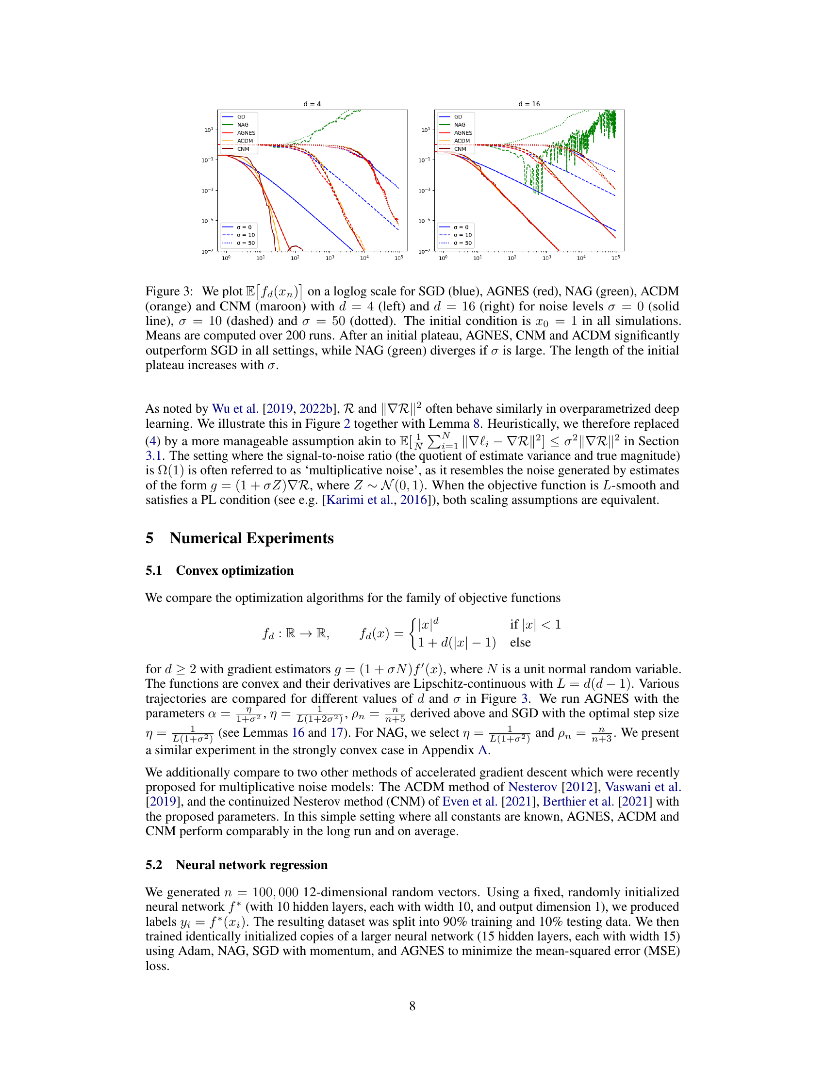
🔼 The figure compares the performance of five optimization algorithms: SGD, AGNES, NAG, ACDM, and CNM on two convex functions with different dimensions (d=4 and d=16) and noise levels (σ=0, 10, 50). It shows that AGNES, CNM, and ACDM significantly outperform SGD, especially at higher noise levels, while NAG diverges for large σ.
read the caption
Figure 3: We plot E[fa(xn)] on a loglog scale for SGD (blue), AGNES (red), NAG (green), ACDM (orange) and CNM (maroon) with d = 4 (left) and d = 16 (right) for noise levels σ = 0 (solid line), σ = 10 (dashed) and σ = 50 (dotted). The initial condition is x0 = 1 in all simulations. Means are computed over 200 runs. After an initial plateau, AGNES, CNM and ACDM significantly outperform SGD in all settings, while NAG (green) diverges if σ is large. The length of the initial plateau increases with σ.
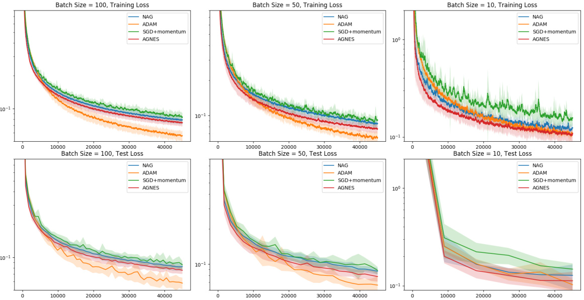
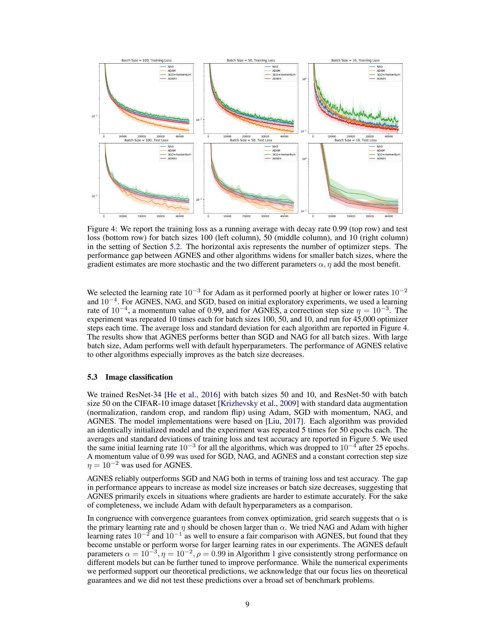
🔼 The figure shows the training and test loss for different batch sizes (100, 50, and 10) using several optimization algorithms: NAG, Adam, SGD with momentum, and AGNES. The x-axis represents the number of optimization steps. The results show that AGNES generally outperforms other methods, especially for smaller batch sizes where the noise in gradient estimates is higher. The benefit of using two separate learning rate parameters in AGNES is highlighted for the cases where the gradient estimates have high stochasticity.
read the caption
Figure 4: We report the training loss as a running average with decay rate 0.99 (top row) and test loss (bottom row) for batch sizes 100 (left column), 50 (middle column), and 10 (right column) in the setting of Section 5.2. The horizontal axis represents the number of optimizer steps. The performance gap between AGNES and other algorithms widens for smaller batch sizes, where the gradient estimates are more stochastic and the two different parameters α, η add the most benefit.

🔼 This figure compares the performance of AGNES against other optimizers (SGD with momentum, NAG, and Adam) for different batch sizes on a neural network regression task. The results are presented as running averages of the training and test losses. The figure shows that AGNES consistently outperforms other methods, especially with smaller batch sizes, where gradient estimates are noisier.
read the caption
Figure 4: We report the training loss as a running average with decay rate 0.99 (top row) and test loss (bottom row) for batch sizes 100 (left column), 50 (middle column), and 10 (right column) in the setting of Section 5.2. The horizontal axis represents the number of optimizer steps. The performance gap between AGNES and other algorithms widens for smaller batch sizes, where the gradient estimates are more stochastic and the two different parameters α, η add the most benefit.

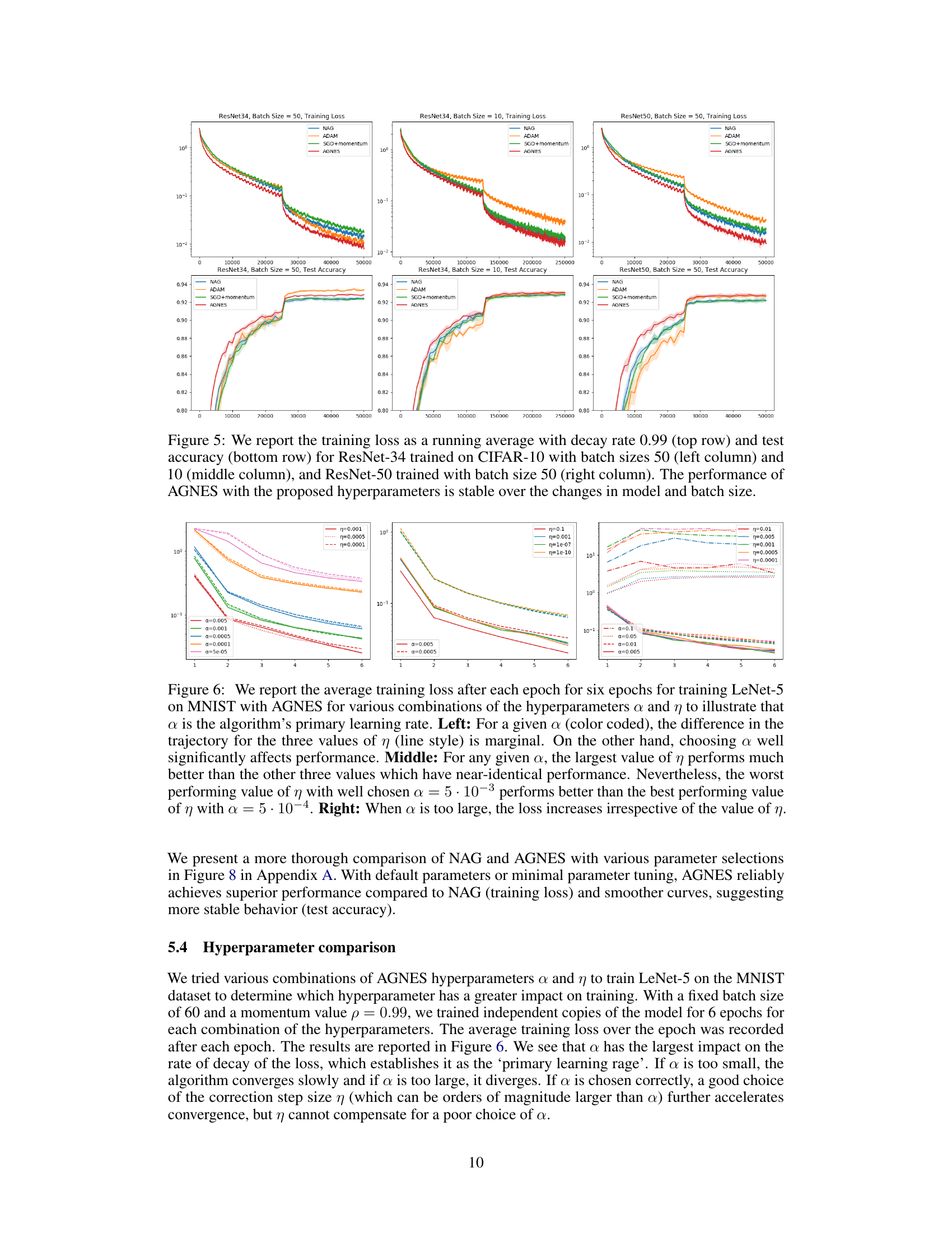
🔼 This figure shows the impact of hyperparameters α and η on the performance of AGNES for training LeNet-5 on the MNIST dataset. The left panel demonstrates that α is the crucial hyperparameter, with variations in η having a smaller effect. The middle panel shows that using the largest value of η is optimal for a given α, while the right panel reveals that very large values of α lead to increased loss regardless of η.
read the caption
Figure 6: We report the average training loss after each epoch for six epochs for training LeNet-5 on MNIST with AGNES for various combinations of the hyperparameters α and η to illustrate that α is the algorithm’s primary learning rate. Left: For a given α (color coded), the difference in the trajectory for the three values of η (line style) is marginal. On the other hand, choosing α well significantly affects performance. Middle: For any given α, the largest value of η performs much better than the other three values which have near-identical performance. Nevertheless, the worst performing value of η with well chosen α = 5·10−3 performs better than the best performing value of η with α = 5·10−4. Right: When α is too large, the loss increases irrespective of the value of η.
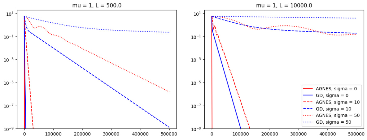
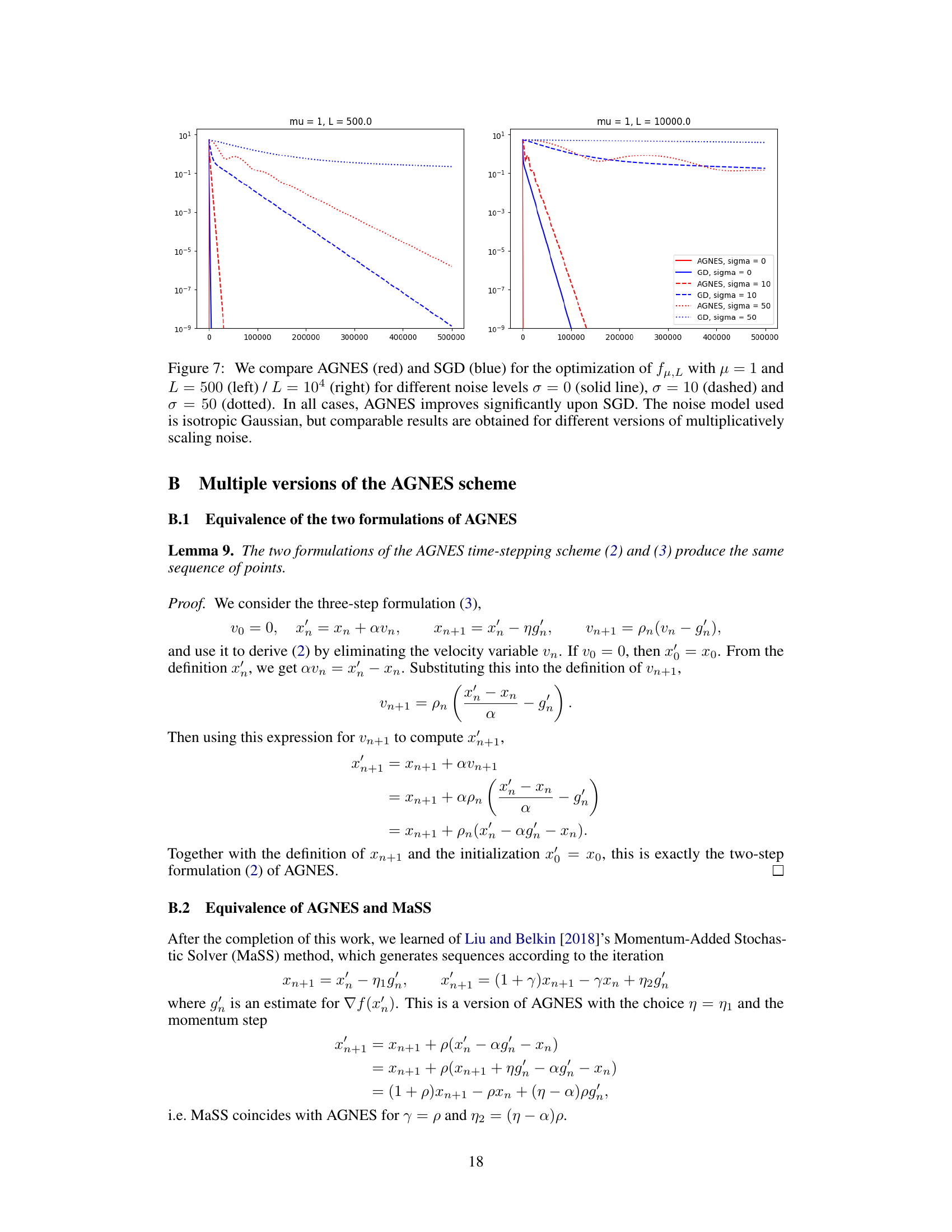
🔼 This figure compares the performance of AGNES and SGD on a strongly convex objective function with varying levels of multiplicative noise (σ = 0, 10, 50). It shows that AGNES consistently outperforms SGD across different noise levels and problem parameters (L=500 and L=10000). The noise is isotropic Gaussian, but similar results were seen with other multiplicative noise models.
read the caption
Figure 7: We compare AGNES (red) and SGD (blue) for the optimization of fμ,L with μ = 1 and L = 500 (left) / L = 10⁴ (right) for different noise levels σ = 0 (solid line), σ = 10 (dashed) and σ = 50 (dotted). In all cases, AGNES improves significantly upon SGD. The noise model used is isotropic Gaussian, but comparable results are obtained for different versions of multiplicatively scaling noise.

🔼 This figure compares the performance of NAG and AGNES on the CIFAR-10 dataset using ResNet34. It shows training loss and test accuracy for various momentum values in NAG, contrasted with the performance of AGNES using default and slightly modified hyperparameters. The results highlight AGNES’s consistent and superior performance across different momentum settings in NAG.
read the caption
Figure 8: We trained ResNet34 on CIFAR-10 with batch size 50 for 40 epochs using NAG. Training losses are reported as a running average with decay rate 0.999 in the left column and test accuracy after every epoch is reported in the right column. Each row represents a specific value of momentum used for NAG (from top to bottom: 0.99, 0.9, 0.8, 0.5, and 0.2) with learning rates ranging from 8.10-5 to 0.5. These hyperparameter choices for NAG were compared against AGNES with the default hyperparameters suggested a = 10-3 (learning rate), η = 10-2 (correction step), and p = 0.99 (momentum) as well as AGNES with a slightly smaller learning rate 5·10-4 (with p = 0.99, η = 10-2 as well). The same two training trajectories with AGNES are shown in all the plots in shades of blue. The horizontal axes represent the number of optimizer steps.
Full paper#
